The Vacuum’s Superfluid Lattice

When the photon is modeled as a vortex dipole in a superfluid substrate, the vacuum’s ≈100 μm lattice size follows from the dark-matter density

Author

Affiliation

Jeff Vroom

Independent

Abstract

This paper proposes that space is filled with a superfluid substrate — the self-binding condensate modeled by Zloshchastiev — and a photon is a modon, the self-propelled counter-rotating vortex dipole known from the ocean and atmosphere. Two consequences follow with no free parameter. First, the smallest modon the substrate can carry is one lattice cell wide, which fixes the cell size from the measured dark-matter density alone: \xi=(\hbar/\rho_\mathrm{DM}c)^{1/4}\approx112\,\mum at unit occupancy. Second, the vortex geometry predicts a pure dimensionless number — the cell occupancy f=4\pi/(K\sqrt2)=0.5666, with K=j_{11}^2+1 built from a Bessel zero — which corrects that length to \xi=\xi_\mathrm{CP}f^{1/4}\approx97\,\mum. Here f is a degeneracy parameter, the n\lambda^3 of condensate physics. With the condensate’s mutual friction, Simeonov’s two-fluid model supplies the Bohm quantum potential as the reaction force of a counter-rotating boundary layer; the charged-lepton Koide relation then follows to 9 ppm, the Higgs vacuum expectation value to 0.06\%, the fine-structure constant to 1.45\%, and c_\mathrm{GW}=c exactly — supplying a fluid mechanism underneath these Standard Model quantities. On cosmological scales gravity becomes an ebbing leak through counter-rotating boundaries, with the stream falling in between: Barceló–Liberati–Visser analog gravity applied to the substrate equations reproduces the Painlevé–Gullstrand (Schwarzschild) metric, Volovik’s self-tuning vacuum supplies a naturally tiny cosmological constant, and the MOND acceleration scale a_0=c\sqrt{G\rho_\mathrm{DM}} follows to \sim3\%, with reductions in both the S_8 and Hubble tensions. The whole gap between the electroweak scale and the lattice is then one pure number, the condensation number \nu=m_\mathrm{eff}/m_1=\xi/\bar\lambda_\mathrm{eff} \approx8.4\times10^8, and it is over-determined. Cosmology plus the geometric f gives \nu=8.35\times10^8; the measured Higgs vacuum expectation value, sharing no input beyond \hbar and c, gives 8.36\times10^8; the fast solar wind lands a third time within 5\%.

Introduction

This paper continues an established thread — that empty space is a superfluid — by adding two adjustments:

1. The quantum potential is a boundary layer. The Bohm quantum potential becomes the reaction force of a superfluid’s counter-rotating boundary layer (following Simeonov).
2. The photon is a modon in that same fluid (Figure 1), following the vortex-dipole solutions of Larichev–Reznik: the self-propelled pair of counter-rotating vortices that oceanographers and atmospheric physicists already know from Gulf Stream rings and the Madden–Julian oscillation. A modon carries energy and momentum but transports no net mass, moves at the speed its medium allows, and is annihilated only by its mirror image — every property a photon must have.

This combines old and new physics into a satisfying result. In 1861 Maxwell built electromagnetism on a sea of molecular vortices, and Thomson’s vortex atom followed in 1867; neither could find a medium that supplies inertia and holds an electron’s orbit. A self-binding superfluid fills that gap, and turns established superfluid physics into equations that span quantum mechanics and general relativity.

From just these — the boundary layer’s mutual friction and reaction force, plus the energy of the smallest modon the fluid can carry (through Planck’s constant) — a single length falls out: the lattice cell size \xi, the Compton wavelength of the vacuum’s particle/vortex. It is fixed by the measured dark-matter density with no free parameters,

\xi_\mathrm{CP}=\left(\frac{\hbar}{\rho_\mathrm{DM}\,c}\right)^{1/4}\approx112\;\mu\mathrm{m},

and the vortex geometry independently predicts a pure dimensionless number — the cell occupancy f=4\pi/(K\sqrt2)=0.5666 — which is the occupancy that length assumed to be 1. Using the close-packing geometry lowers the size to the accurate value, \xi=\xi_\mathrm{CP}f^{1/4}\approx97\;\mum.

That one length, with the vortex geometry, then finds:

Quantity	Framework	Observed	Off by	Status
Higgs vacuum expectation value	246.07 GeV	246.22 GeV	0.06\%	the \nu row read forwards — the same agreement, not a second one
Koide lepton relation Q	2/3	0.666660	9 ppm	derived — zero free parameters
MOND scale c\sqrt{G\rho_\mathrm{DM}}	1.16\times10^{-10}	1.20\times10^{-10}	\sim3\%	anchored to \nu
Fine-structure constant \alpha	1/135.1	1/137.04	1.45\%	tree-level; the correction is an open problem
Gravitational-wave speed c_\mathrm{GW}	c	c	<10^{-14}	derived — zero free parameters
Condensation number \nu	8.348\times10^8	8.358\times10^8	0.12\%	derived — geometry +\,\rho_\mathrm{DM}, checked against the measured VEV

That length is \xi, the lattice cell size: a \approx100\,\mum structure filling all space that transmits light losslessly, has no hard floor, and couples to chemistry seamlessly. Hiding in plain sight.

The framework uses five established results:

• Volovik, The Universe in a Helium Droplet (Volovik 2003) — superfluid ^3He reproduces fundamental properties of the vacuum at both atomic and galactic scales, including an emergent relativistic (Dirac) spectrum.
• Zloshchastiev and collaborators (Zloshchastiev 2020; Avdeenkov and Zloshchastiev 2011) — a self-binding condensate whose logarithmic equation of state (the superfluid-vacuum model) has a Lorentz-invariant ground state.
• Bush, Oza and collaborators (Bush and Oza 2020) — a droplet bouncing on a vibrating bath, a particle in self-generated resonance with a responsive substrate, experimentally reproduces quantized orbits, tunneling, and single-particle diffraction.
• Simeonov (Simeonov 2025) — the Madelung/Bohm quantum potential follows from the material derivative of the osmotic velocity in a two-fluid model.
• Khoury and Berezhiani (Khoury 2015; Berezhiani and Khoury 2015) — if dark matter is a superfluid, its phonons mediate a MOND-like force on galactic scales, with a sharp transition to ordinary cold-dark-matter behavior above a critical velocity.

To find the quantum potential, Simeonov’s two fluids fit perfectly as the two components of a superfluid: the co-rotating bulk is the condensate, and his counter-flowing second fluid is the counter-rotating component of the Hall–Vinen–Bekarevich–Khalatnikov (HVBK) mutual-friction force.

The photon as a modon (Figure 1) travelling at the speed of light requires a substrate with a proportional rotational velocity. The modon’s Bessel match function then finds the lattice size from the smallest modon the substrate can support.

Figure 1: The photon as a modon. A modon is a bound pair of counter-rotating vortex cores — here +\omega (counter-clockwise) above -\omega (clockwise) — sharing a single closed envelope of streamlines of scale \xi. Each core sits in the velocity field of the other, so the pair advects itself forward (the induced jet between the cores) and travels through the substrate at the signal speed c without the substrate doing net work. Because the two spins are equal and opposite, the substrate mass each core would carry cancels exactly (\int\psi\,\mathrm{d}A=0): the modon transports no net mass and is therefore massless, even though the pattern propagates at c carrying energy E=h\nu and momentum p=E/c — exactly the properties a photon must have.

The cosmological route cleanly shows the lattice cell size from the measured dark-matter density and the constants \hbar and c alone — \xi_\mathrm{CP}\approx112\,\mum (Equation 8), four measured inputs, no free parameter.

A clear geometry prediction, the cell occupancy f=4\pi/(K\sqrt2)=0.5666 (Equation 10) adjusts the cell size to the true value. Its three factors are three separate physical requirements on one medium — the 4\pi that lets the lattice gravitate, the 1/K that lets it carry photons, the 1/\sqrt2 that makes it a real condensate — and none of them is adjustable. Using this fraction instead of 1 gives \xi=\xi_\mathrm{CP}f^{1/4}\approx97\,\mum (Equation 11).

Particle physics finds the same size with dark matter density using the effective quantum’s reduced Compton length \bar\lambda_\mathrm{eff}=\hbar/(m_\mathrm{eff}c)=116\,fm, that uses \sin^2\theta_W and m_e, and the pure number of those rulers that fit in one cell — the condensation number \nu=m_\mathrm{eff}/m_1\approx8.4\times10^8 (Equation 12). Three measurements that share no physics land on that one number: cosmology through the geometric f, the measured Higgs vacuum expectation value, and the measured fast-solar-wind onset. The first two agree to 0.12\% (§2.2).

The lattice size is further confirmed through many fuzzy matches: the substrate and its lattice hide from observation through smooth energy transport and the lack of a hard floor. Still, enough measurements align — fenced in from cosmology, the electroweak scale, molecular geometry, and the far-IR sky — to give confidence in the \approx100\,\mum size, which supports numerous softer predictions (§5).

Understanding the results

This section puts the math of §1 in a context that is easier to picture.

The lattice size, \xi \approx 100\;\mum, feels at first glance far too large — the natural objection is that a structure that big filling all space would have been seen. The rest of this section is the answer to that objection.

Picture \xi not as a rigid grid but as the perturbation envelope of a stiff superfluid spinning at \approx 0.776\,c (the substrate’s own inner rotation speed, c\sqrt{2\alpha_{mf}}, §1.1.1). It mimics a vacuum but is nothing like one. It is an energetic, closely packed, extremely coupled BEC condensate formed from balanced vortices breathing in anti-phase, tied together by topologically protected vortex lines. Its particles move too fast and sit too close to be resolved as individuals; instead they form lines connected to a vortex core, which disconnect and reconnect. As disconnected lines they bounce and rebound at the Compton wavelength. With an anti-phase partner they form counter-spinning nesting eddies, while retaining a quantized momentum that returns them to the connected state along a path that is very hard to break. That stiffness is what lets them bend quickly enough to transmit modons — radiation without energy loss. Counter-spinning boundary layers form around the electron’s orbit and keep it from collapsing. Those same stiff layers limit the leak we feel as gravity, and between them the stream falls.

And the stiff substrate provides the energy that supports photons as self-advecting modons. Neutrinos are bare vortices wrapped in a modon dressing and move the same way. Everything else pushes a bow wave, trails a balancing stern wave — at steady speed the two cancel and it coasts without substrate drag, vacuum-like inertia. Only near the signal speed, c, does the bow wave stiffen into ram pressure.

The substrate has two other speed limits. When an electron nears the inner one — the rotational speed of the substrate, \approx 0.776\,c — its boundary tears and spits out a gamma modon near 300 keV, seen as a lightning bolt, a solar flare, or a tokamak disruption.

When an organized current like the Sun’s polar wind hits the outer-rim limit near 750 km/s, v_L, it spills vortices carrying the excess energy. A galaxy’s slow swirl, well below 750 km/s, stays coherent — modified gravity, MOND’s extra grip. But two clusters slammed together above that speed create shear, and the substrate acts like an ordinary collisionless gas, streaming through itself — seen as dark matter.

The lattice cell size is large for a simple reason: through the Compton wavelength, lighter particles have longer wavelengths, and dc1 is very light. Its cell vortex’s lines start crowded at a core, disconnect, and oscillate outward at \sim0.776\,c — frictionlessly, so every collision is perfectly elastic — before reconnecting a wavelength later. A lighter, less dense core sends its ripples farther per cycle and overlaps more deeply with its anti-phase breathing partner, so the pair needs a larger envelope before a containing counter-spinning boundary can close around it.

That envelope is what the condensation number \nu=m_\mathrm{eff}/m_1\approx8.35\times10^8 measures — one pure number wearing two faces. As a mass count, \nu is the number of dc1 quanta that condense in concert to make one effective quantum — the 1.70 MeV vortex unit inside every particle. As a length count, the same number is the Compton lift \xi/\bar\lambda_\mathrm{eff} — how many effective-quantum reach-lengths (116 fm) fit across one lattice cell. The Compton length shows longer wavelengths for less mass. That sheer size is where the substrate’s energy hides, and it has a measured mirror. In ^3He, the substrate’s closest analog, a single Cooper pair’s coherence envelope already spans \sim10^6 atoms — possible only in a strongly overlapping BCS condensate. The ^3He count shares the mechanism — a light constituent has a long Compton reach, so the coherent envelope dwarfs the constituent spacing — but not the quantity: a condensate of far lighter cores, coupled even more strongly, reaches \approx8.35\times10^8 (developed in §2.2).

All of these disconnecting and reconnecting vortex lines make the substrate an energetic seamless glue, underlying it all and imposing a large blurry window for observations. It hides further still by nesting inside stable, balanced layers, concealing a subtle scale-invariant organization formed by the substrate energy.

The substrate overview comes first, for grounding, followed by the backbone equations. The shape of the lattice then covers how boundary layers are influenced through chemistry, and the paper closes with the substrate predictions, the open problems, and the conclusion.

The substrate overview

The framework posits a new particle, nicknamed dc1¹, of mass m_1\approx2\;\mathrm{meV}/c^2. It condenses into an extremely coupled BCS condensate and forms the quantized vortices that carry the substrate’s internal weather; because its self-interaction is logarithmic it also self-binds into a lattice of cell size \xi.

These identifications follow:

• The vacuum is the dc1 condensate, organized into a lattice of cell vortices — about one self-bound dc1 wavefunction per cell, each breathing anti-phase with its counter-rotating partner. Its rest-frame density is the cosmological dark-matter density, n_1 m_1 = \rho_\mathrm{DM}.
• Mass is leaking rotational kinetic energy — the fraction of a vortex’s spin that escapes its outermost counter-rotating boundary, the rest staying trapped and unweighable (§1.1.1).
• A fermion (electron, quark) is a persistent particle vortex of dc1, a topologically protected excitation, with an odd number of counter-rotating boundary layers separating its co-rotating interior from the surrounding substrate. The boundary count is what makes it a fermion.
• A boson (photon, W, Z) is a balanced, counter-rotating pair — a modon for the photon — with even boundary parity and zero net forward momentum, hence massless or massive only through its internal binding.
• A proton is a Borromean ring, three locked vortices — two up quarks and one down. Colors come from topological interlocking phases, and flavors from braids of the knot.
• Spin statistics — counter-rotating boundary-layer angular momentum, with a two-layer, double-cover topology, gives the 720° return.

From there, the bridge equation helps build the backbone of the hydrodynamic model of the lattice, which then yields a number of predictions — close fits to several observations, and added clarity for many others.

The argument runs in four steps:

1. Shows the quantum potential as the reaction force of the counter-rotating boundary layer.
2. Uses the photon’s minimum energy as a modon to fix the bridge equation.
3. Extends that picture to gravity, as a slow leak of substrate through the same boundary.
4. Works out the lattice’s vertical geometry and shows the clear patterns of underlying organization the substrate reveals.

A closing section gathers the framework’s predictions and its open problems.

1 Counter-rotating layers and the quantum potential

Start with the substrate at rest and ask what happens around an organized disturbance — a vortex, or an orbiting structure. A co-rotating region of dc1 flow has, at its edge, a shear zone; in a low-dissipation superfluid the lowest energy path to absorb that shear is a thin counter-rotating boundary layer of eddies (Figure 2). This decomposition — a co-rotating bulk and a counter-rotating boundary — is the two-fluid structure of HVBK superfluid hydrodynamics, and it is the structure Simeonov’s model needs.

Figure 2: The shear zone: where counter-rotation comes from. Left: a single co-rotating dc1 core (+\omega, blue) sits in the resting substrate; at its rim the flow must fall back to the still fluid, and the cheapest way to close that velocity jump is a thin counter-rotating skin (-\omega, red) — a shielded vortex whose total circulation cancels to zero (\int\psi\,\mathrm dA=0). Centre: zoom into the seam — two regions in relative motion put a single roller between them, spun the opposite way to the bulk; that is the whole mechanism. Right: the velocity profile makes it inevitable. The azimuthal speed v_\theta rises through the core (solid-body rotation, \omega=+2\Omega) to a peak at the rim, then drops back toward zero faster than the 1/r tail an unshielded vortex would keep; wherever v_\theta falls faster than 1/r the vorticity flips sign (\omega<0) — that is the skin — and the net circulation returns to zero. This one primitive recurs throughout: wrapped on an orbital it becomes the quantum potential (Figure 3); set core-to-core it is the photon (Figure 1).

Let fluid 1 (co-rotating, the “particle”) have density \rho_1 and velocity \mathbf v_1, and let fluid 2 (counter-rotating boundary) respond to gradients in fluid 1 with an osmotic velocity

\mathbf v_2 = -D\,\nabla \ln\rho_1, \qquad D = \frac{\hbar}{2m}, \tag{1}

where D is the diffusion constant of the counter-rotating layer. Simeonov (Simeonov 2025) shows that the reaction force of fluid 2 back on fluid 1 is, with R=\sqrt{\rho_1},

\mathbf F_\mathrm{reaction} = -\nabla Q, \qquad Q = -\frac{\hbar^2}{2m}\,\frac{\nabla^2 R}{R}, \tag{2}

which is the Bohm quantum potential.² It is the back-pressure of that same skin on the curvature of the co-rotating density — applied to the hydrogen orbital (Figure 3). The three behaviors follow: near a density maximum \nabla^2 R<0 so Q>0 — a repulsive “quantum pressure” that keeps the electron from spiralling in; near a node Q dips sharply negative and its gradient pushes flow away from the node, maintaining it; in a uniform region \nabla^2R=0 and Q=0, no boundaries, no quantum effects. This is the substrate content of Bush’s hydrodynamic analogy: the electron is a real structure resonating with a real responsive substrate, and the “pilot wave” is the dc1 flow that the counter-rotating layer organizes around it.

Figure 3: The quantum potential as a boundary-layer back-pressure. Left: a hydrogen 1s electron is a co-rotating vortex of dc1 (+\omega, blue) whose density \rho_1 peaks at the proton and falls off outward — a slice of the n=1 orbital. Where the co-rotating flow shears against the resting substrate, the cheapest response is a thin counter-rotating boundary layer of eddies (-\omega, red — fluid 2), which tracks gradients in \rho_1 with the osmotic velocity \mathbf v_2=-D\,\nabla\ln\rho_1, D=\hbar/2m. Right: the reaction force of that layer back on the bulk is exactly the Bohm quantum potential Q=-\frac{\hbar^2}{2m}\nabla^2R/R (with R=\sqrt{\rho_1}). Near the density peak \nabla^2R<0, so Q>0: an outward “quantum pressure.” For the ground state it exactly cancels the inward Coulomb potential V=-e^2/r, leaving the sum V+Q=E constant — the substrate reason the electron neither spirals in nor radiates.

1.1 Where \hbar comes from

In Equation 1 the diffusion constant D=\hbar/(2m) used Planck’s constant. Here we meet it again, this time in an equation built from vortex mechanics. The HVBK mutual-friction force is built with a dimensionless coupling \alpha_{mf} — the fraction of each boundary interaction that dissipates energy rather than deflecting the flow. For a superfluid with quantized circulation \kappa_q = h/m_\mathrm{eff}, the effective diffusivity of vortex-mediated transport is D_{sf} = \kappa_q/(4\pi\,\alpha_{mf}).³ Setting this equal to the quantum diffusion constant D=\hbar/(2m) of Equation 1 — where m is the mass of the particle the orbital builds (the electron, for hydrogen) — and substituting \kappa_q = 2\pi\hbar/m_\mathrm{eff} gives the central mass relation

\boxed{\;m_\mathrm{eff}\,\alpha_{mf} = m\;} \tag{3}

and, equivalently, \hbar = 2mD. Planck’s constant comes from the action of the counter-rotating boundary layer. It is the discrete minimum vortex circulation, the circulation quantum of the substrate, m_\mathrm{eff}\kappa_q, where m_\mathrm{eff} is the mass of one effective quantum of dc1 circulation and \alpha_{mf} is the mutual-friction coupling for the relevant scale. With the electroweak value \alpha_{mf} = \tan^2\theta_W = \sin^2\theta_W/(1-\sin^2\theta_W) = 0.3008⁴ and m=m_e, the electron mass, the effective quantum is m_\mathrm{eff} = m_e/\alpha_{mf} = 1.70\;\mathrm{MeV}/c^2, heavier than the electron by 1/\alpha_{mf}\approx3.3. Applying the same relation in the nuclear sector, with this one shared quantum, shows the proton coupling \alpha_{mf}^{(N)} = m_p/m_\mathrm{eff}\approx552: the proton is \sim552 effective quanta of the same substrate unit, the electron a 0.3008 fraction of one.⁵

1.1.1 E=mc^2 - vortex energy fully expressed

A particle “at rest” is a parcel of substrate spinning in place — ordinary rotational kinetic energy. Only part of that is visible, because the inner energy is trapped behind the counter-rotating boundary layer that forms in the region right around the particle. The inside part hides; only the leak shows up in observations. The leaking fraction is \alpha_{mf}: about 30\% of the effective quantum’s spin energy dissipates outward. The other \approx70\% stays reactive and invisible to weighing — but not invisible to a hard enough probe, where it shows up as the scattering phase and the magnetic moment (§5.6).

But together, the flywheel energy of the spin and the leak combined have a speed, the speed of the medium, c, and the rim is locked to a fixed fraction of it, v_\mathrm{rot}^2 = 2\alpha_{mf}c^2 (v_\mathrm{rot}=0.776\,c, the substrate’s own inner rotation speed). So

\underbrace{\tfrac12\,m_\mathrm{eff}\,v_\mathrm{rot}^2}_{\text{flywheel energy stored}} \;=\; \tfrac12\,m_\mathrm{eff}\,(2\alpha_{mf}c^2) \;=\; \underbrace{(\alpha_{mf}\,m_\mathrm{eff})}_{\text{the part that leaks}}c^2 \;=\; m_e c^2 . \tag{4}

The \tfrac12 and the 2 cancel; \alpha_{mf} converts the effective quantum into the observed electron mass; what is left is E=mc^2. The c^2 is the flywheel’s rim speed, pinned to c because c is the fastest the substrate carries anything. And mass is not converted into energy: mass is that energy, seen through the finite aperture of a counter-rotating boundary. A nuclear reactor does not convert mass to energy, it tears open the stiff barrier that fixes the aperture, exposing the vast rotational energy that is already there.

The factor \alpha_{mf}=\tan^2\theta_W comes from the Weinberg angle, measured in particle accelerators, and the same coupling runs both sectors. The electron’s narrow 0.3008 lets out under a third of one quantum’s spin, which is why it is light. The proton’s \alpha_{mf}^{(N)}\approx552 is a wide aperture, which is why \sim99\% of its mass is boundary energy — and why a bound nucleus weighs less than its parts, since two merged boundaries present a smaller leaking surface than two separate ones. One measured coupling, read at two scales, and the mass of ordinary matter becomes a statement about how much of the substrate’s spin each boundary lets escape.

The shared effective quantum m_\mathrm{eff} is fixed by Equation 3 from m_e and \alpha_{mf}. It will matter in Step 2, because the same circulation quantum \kappa_q = 2\pi\hbar/m_\mathrm{eff} sets the speed of light and the modon’s action.

2 The photon as a modon, and the bridge equation

2.1 The modon and the emergent speed of light

A modon is a steadily propagating dipole of two counter-rotating vortex cores that advect each other forward: each core sits in the velocity field of the other, and their mutual induction drives the pair through the substrate without the substrate doing net work (Larichev and Reznik 1976; Saffman 1992). Its energy is entirely internal, its net mass transport is zero, and it is destroyed only by meeting an anti-modon. These are exactly the properties a photon must have: massless, self-propelled, energy E=h\nu, annihilated by its antiparticle.

Those same counter-rotating layers from the previous section show why the photon is a modon and how the atom emits one (Figure 4). A bound orbital is built from the standing wave’s counter-spinning shells. When the electron drops from n\to n', the released energy \Delta E=E_n-E_{n'} has to go somewhere: it thins the seam between two shells, that sheared layer rolls up into a counter-rotating pair, and the pair pinches off as a free modon carrying \Delta E=h\nu. The photon is born massless and moving at c based on the orbital’s own rotation speed — each direction rotating at 0.776\,c.

Figure 4: How an atom emits a photon: a modon pinches off. (I) A bound orbital is built of the standing wave’s counter-spinning shells — an inner co-rotating shell (+\omega, blue) and an outer counter-rotating shell (-\omega, red), the same two-fluid pairing that supplies the quantum potential (Figure 3). (II) When the electron drops n\to n', the released energy \Delta E=E_n-E_{n'} has nowhere to hide: the seam between the two shells thins where their shear concentrates. (III) That sheared layer rolls up, Kelvin–Helmholtz fashion, into an embryonic counter-rotating vortex pair. (IV) The pair pinches off as a free modon and self-advects at the substrate speed c, carrying \Delta E=h\nu away while the atom settles into the smaller n' orbital. The freed pair is the orbital’s own two counter-spinning shells, now detached — +\omega above, -\omega below — which is why a photon is born already massless (\int\psi\,\mathrm{d}A=0) and already moving at c.

In the strong-coupling BEC regime the dc1 quasiparticle spectrum is Dirac-like,

E^2 = \mu^2 + c^2 p^2, \qquad c = \frac{\hbar}{m_1\,\xi} \tag{5}

with a single isotropic speed set by the dc1 mass and the coherence length \xi (Volovik 2003).⁶ Every low-energy excitation — phonon, modon, and the tensor metric perturbation of Step 3 — inherits this one speed, so the framework predicts c_\mathrm{GW}=c exactly; gravity should travel at the speed of light. And this matches the result from the gravitational wave measured by LIGO, GW170817: |c_\mathrm{GW}/c-1| < 6\times10^{-15}. The speed of light is the maximum group velocity of organized disturbances in a superfluid of 2\;\mathrm{meV} particles with a hundred-micron coherence length.

The symbol \xi is the coherence length of the dc1 condensate - the perturbation envelope of the photon/modon that comes from Volovik’s superfluid helium, using the speed of light as the medium speed. This same equation is also the Compton wavelength formula using the dc1 particle’s mass. And with the close-packing nature of this densate, the length is also the lattice cell size.

The modon has a precise solution from Larichev–Reznik (Larichev and Reznik 1976) that matches the interior and exterior boundary energies, observed from long-lived eddy pairs in the ocean and atmosphere. Inside a critical radius the flow circulates and oscillates; outside it dies away exponentially into the surrounding substrate; and the two must join smoothly at the edge of the cell, r=\xi. Picture a self-contained swirl with a sharp skin — trapped circulation within, a fading halo without.

The interior pattern is a Bessel function, \psi\sim J_1(pr), for the same reason a circular drumhead vibrates in Bessel-function modes: it is the natural shape of a wave confined to a disk. Requiring the lowest mode — the swirl completing exactly one lobe across the cell, with nothing left over — pins the interior wavenumber to the first zero of J_1, the pure number j_{11}=3.8317 (the same constant that sets the fundamental dipole tone of a clamped circular drum). The exterior halo, \psi\sim K_1(qr), decays over exactly one coherence length, q\xi=1. Matching the two smoothly at the skin combines them through p^2+q^2; in units of the cell size (multiplying by \xi^2) this becomes the dimensionless structure constant⁷

K = (p\xi)^2 + (q\xi)^2 = j_{11}^2 + 1 = 15.68 . \tag{6}

K is a pure geometric number, like \pi — the square of a Bessel zero plus one, carrying no units and taking the same value in every unit system. The term j_{11}^2 is the lowest mode where the interior wavelength matches the cell’s wavelength. The term +1=(q\xi)^2 is the exterior tail over exactly one coherence length (q\xi=1), and both are fixed by the single scale \xi=\hbar/(m_1c), so the “+1” is a consequence of the cell size, not a free shift. Setting the resulting modon speed equal to c recovers the Volovik relation c=\hbar/(m_1\xi): modon matching is not a new assumption but the statement of why a counter-rotating dipole in the substrate travels at exactly the speed of light.

Two existence conditions follow. First, the matching has no solution below scale \xi: the smallest modon is exactly one lattice cell wide. Second, that smallest modon has wavelength \lambda=\xi; since a modon carries energy E=hc/\lambda, this fixes a minimum energy

E_\mathrm{min} = \frac{hc}{\xi} = 2\pi\,m_1 c^2 \approx 12.8\;\mathrm{meV}, \tag{7}

the minimum energy of a single localized modon — one whose whole dipole fits in one cell — at \lambda\sim100\,\mum, \nu\sim3 THz. This is a floor on one elementary modon, not a cutoff on the spectrum: lower-frequency light propagates as a coherent superposition of many cells, the collective limit of the same modon field (§5.2).⁸

How, then, does ordinary light live above this floor? Visible light (\sim2 eV) sits far above threshold, \lambda\ll\xi: it keeps the full \xi-scale envelope but concentrates its energy in a compact sub-cell dipole core — a boat in a harbor, a small hull trailing a basin-wide wake. At the floor the hull grows to fill the harbor, and core and envelope coincide at \xi. Below it (\lambda>\xi) the dipole can no longer localize inside one cell, and the excitation spreads into a delocalized, many-cell collective mode — the way radio, microwave, and the CMB propagate, each photon a single quantum of collective winding spread over many cells, just as a long-wavelength phonon is one quantum of collective motion far below any single atom’s vibration. So 12.8 meV (\sim3 THz) is a crossover in modon structure, not an edge in the spectrum: nothing goes dark there, only the shape of the packet changes.

2.2 The bridge equation

The next step is to find the lattice size \xi. From cosmology, the dark-matter density gives a larger size that the cell occupancy adjusts down. From particle physics, the same size arrives as a count — the condensation number \nu — and several independent observations land on it.

Route 1 — from cosmology. Three relations that describe the nature of the dc1 superfluid: the Volovik speed Equation 5, the composition n_1 m_1 = \rho_\mathrm{DM}, and close-packing n_1\xi^3 \approx 1 (one condensate wavefunction per cell, the Bose-condensation degeneracy condition n\lambda_{dB}^3\sim1).⁹ Eliminating n_1 and m_1 leaves a single equation,

\xi_\mathrm{CP} = \left(\frac{\hbar}{\rho_\mathrm{DM}\,c}\right)^{1/4} \approx 111.8\;\mu\mathrm{m}, \tag{8}

with inputs \hbar, c, and the dark-matter density \rho_\mathrm{DM}=2.254\times10^{-27}\;\mathrm{kg/m}^3 from Planck 2018 (Planck Collaboration et al. 2020).¹⁰ (Equivalently n_1\xi^3=1 and Equation 5 reduce, with no numbers, to \rho_\mathrm{DM}\xi^3=m_1 — close-packing is the same statement as emergent light.)

Route 2 — the electroweak side from a pure number. Using two conditions on the vortex lattice — the modon-matching condition Equation 6 and a gravitational self-consistency condition called SC2 — together with the Gross–Pitaevskii core balance shared with Route 1. The thing to hold onto is that not one of the three is a length equation. Read honestly they are a normalization, a shape, and an energy balance, and what they assemble into is a dimensionless number.

SC2 is the requirement that the lattice not merely carry disturbances but gravitate — that a lump of substrate energy bend the emergent (acoustic) metric exactly as Newton says a mass should, \nabla^2\Phi = 4\pi G\rho (Step 3). The 4\pi comes from the surface area of a unit sphere, the Gauss solid angle over which flux from a point spreads in three dimensions. For the substrate’s vortices to source gravity with that coefficient, one circulation quantum must satisfy

\kappa_q\,\Omega_v = 4\pi c^2, \qquad \Omega_v = \frac{2m_\mathrm{eff}c^2}{\hbar}, \tag{9}

where \kappa_q=2\pi\hbar/m_\mathrm{eff} is the quantum’s circulation — its swirl, in m²/s — and \Omega_v is its Compton zitterbewegung clock, its internal rate in 1/s. The striking part is that their product is 4\pi c^2 identically: m_\mathrm{eff} cancels. So SC2 adds no adjustable dynamics — it is the statement that the same quantum which carries circulation also sources gravity, and the two roles can only lock together through the geometric 4\pi. Both sides have units m²/s², so SC2 is dimensionally clean and unit-invariant, and it is what hands the cell occupancy its leading 4\pi (Equation 10, §2.3).¹¹ Written out in the lattice’s own variables it reads \Omega_v\,\xi/c = 2\nu — a pure number set equal to a pure number — which is the first sign that this side of the bridge is not going to hand us a length.

The third ingredient is the Gross–Pitaevskii core balance. At a vortex core the condensate’s kinetic energy \hbar^2/(2m_1\xi^2) balances its interaction energy m_1c^2; equating the two fixes the healing length \xi_\mathrm{GP}=\hbar/(\sqrt2\,m_1c)=\xi/\sqrt2 (Fetter 2009). The \sqrt2 comes from the 2 in the kinetic operator \hbar^2/2m — an elementary fact of non-relativistic quantum mechanics.

The three assemble into a fraction. SC2 contributes its Gauss’s-law 4\pi; modon matching contributes 1/K with K=j_{11}^2+1; the core balance contributes 1/\sqrt2. Their product is the cell occupancy, the number of dc1 wavefunctions the substrate actually puts in one cell:

\boxed{\;f = \frac{4\pi}{K\sqrt2} = 0.5666\;} \tag{10}

4\pi is a solid angle, K is a Bessel zero squared plus one, \sqrt2 is the 2 in \hbar^2/2m. This is the bridge equation, and the physical reading of its four factors — including the \eta=1 that says no three-dimensional correction is needed — is §2.3.

Route 1’s close-packing “\approx1” finds the f\!=\!1 idealization: one wavefunction exactly filling each cell. But a real cell is not merely a census volume. Binding energy pulls the cores into overlap, and the modon envelope must close inside the same width. The geometry shows the real occupancy as f, and since \rho_\mathrm{DM}\,c\,\xi^4/\hbar=f makes \xi\propto f^{1/4}, the true lattice cell width

\xi = \xi_\mathrm{CP}\,f^{1/4} = 111.8\;\mu\mathrm{m}\times0.8676 = 97.0\;\mu\mathrm{m}. \tag{11}

Its inputs are \rho_\mathrm{DM}, \hbar, c, and the Bessel zero j_{11} — no free parameter.

The cell occupancy 0.5666 is three conditions held at once: heal a vortex core (1/\sqrt2, Gross–Pitaevskii), close the modon envelope (1/K, Bessel match), and present the correct flux to gravity (4\pi, Gauss).

The other thing the electroweak side supplies is the effective quantum, m_\mathrm{eff}=m_e/\alpha_{mf}=1.699 MeV/c^2 (Equation 3), whose reduced Compton length \bar\lambda_\mathrm{eff}=\hbar/(m_\mathrm{eff}c)=116.2 fm is the ruler the cell is measured in. The one number left over is the count of rulers — the condensation number,

\boxed{\;\nu \equiv \frac{m_\mathrm{eff}}{m_1} = \frac{\xi}{\bar\lambda_\mathrm{eff}} = \frac{\omega_\mathrm{eff}}{\omega_1} \approx 8.35\times10^8\;} \tag{12}

— a ratio of two masses, of two lengths, or of two frequencies, a dimensionless value.¹² Equivalently, as a length set by a length,

\xi = \nu\,\bar\lambda_\mathrm{eff}, \tag{13}

which is [\text{m}]=[\text{m}] and unit-invariant. So Route 2 helps explain the nine-decade gap between the electroweak scale and the lattice cell with this number, using measurements that support it. The cell is large because \nu is large: a very light core sends its ripples far per cycle, and the pair needs a wide envelope before a counter-spinning boundary can close around it.

The value \nu is one pure number with two faces. Inside a particle, \nu is a mass count: 8.35\times10^8 dc1 quanta acting in concert as one effective quantum — a collective occupation number, like the macroscopic occupation of a laser mode. In the resting vacuum, the same number is a length ratio — the Compton lift \xi/\bar\lambda_\mathrm{eff} of Equation 13 — and counts nothing you could point to: a lattice cell holds about one delocalized dc1 wavefunction (the cell occupancy f, Equation 14 below), not 10^8 constituents. They come together in the Compton wavelength formula. So the relationship comes not as a count of particles in an envelope, but a similar lift from from its constituent quantum (2 meV) to its universal condensation unit (1.70 MeV).

And \nu not only supports the cell size, it also finds the Higgs VEV. The chirality-ordered ground state has amplitude v=\sqrt{8\pi\,m_\mathrm{eff}^2c^4\,\nu} — the relativistic Bose amplitude law, with the same gravitational 8\pi=2\times4\pi the substrate uses to gravitate (§5.2) — so the measured v=246.22 GeV inverts to \nu=v^2/(8\pi m_\mathrm{eff}^2c^4). A third measurement supports this value from the heliosphere: the Landau critical velocity v_L=c\,(4\pi/\nu)^{1/3}, from the fast solar wind (§3.3). Both clean reads from the pure energy you’d expect to find in the substrate.

Written as a close-packing statement rather than a count, the same content is the cell occupancy with the “\approx1” made honest:

f \equiv \frac{\rho_\mathrm{DM}\,c\,\xi^4}{\hbar} = \left(\frac{\xi}{\xi_\mathrm{CP}}\right)^4 , \tag{14}

the number of dc1 wavefunctions in one cell.¹³ Cosmology supplies the left side from the size; the geometry of Equation 10 supplies the right.

f is a degeneracy parameter of condensate physics, the count of wavefunctions per cell.

2.2.1 The agreement

The cosmology side and the electroweak side share no parameter beyond \hbar and c — one uses cosmological data (\rho_\mathrm{DM}), the other electroweak physics (\sin^2\theta_W, m_e, and the measured Higgs VEV v). They meet on \nu, and three measurements that share no physics fix it:

Leg	Relation	Measured input	\nu
Cosmology \times geometry	\nu=\xi_\mathrm{CP}f^{1/4}/\bar\lambda_\mathrm{eff}, f=4\pi/(K\sqrt2)	\rho_\mathrm{DM} (Planck 2018)	8.348\times10^8
Electroweak	\nu=v^2/(8\pi\,m_\mathrm{eff}^2c^4)	v=246.22 GeV (collider)	8.358\times10^8
Heliospheric	\nu=4\pi\,(c/v_L)^3	v_L=751.5 km/s (Ulysses)	7.98\times10^8

Cosmological density, collider electroweak physics, and heliospheric flow converge on one \nu\approx8.2\times10^8 to \sim5\%, and the two tightest legs agree to \mathbf{0.12\%}.¹⁴ The two sides use the effective quantum with opposite powers — \nu\propto m_\mathrm{eff} on the length side (through 1/\bar\lambda_\mathrm{eff}), \nu\propto m_\mathrm{eff}^{-2} on the VEV side — so m_\mathrm{eff} cannot cancel out of the comparison. Their agreement is a constraint tying \rho_\mathrm{DM}, v, and \sin^2\theta_W together.

Four supporting data points combine into one match:

• as the pure number, \nu=8.348 vs 8.358\times10^8 — 0.12\%;
• as a length, \xi=97.0 vs 97.1\,\mum — the electroweak cell \nu\,\bar\lambda_\mathrm{eff} against the cosmological \xi_\mathrm{CP}f^{1/4};
• as the cell occupancy, the geometric 0.5666 against 0.5694 — 0.5\%, comfortably inside Planck’s \sim1\% on \rho_\mathrm{DM};¹⁵
• and read forwards rather than backwards, as the Higgs VEV: v=\sqrt{8\pi\,m_\mathrm{eff}^2c^4\nu}=246.07 GeV against the measured 246.22 — 0.06\% (§5.2).

Figure 5: One number, reached three ways. The cosmology route (\rho_\mathrm{DM},\hbar,c) sets the naive cell \xi_\mathrm{CP}=111.8\,\mum at unit occupancy; the zero-parameter geometric cell occupancy f=4\pi/(K\sqrt2)=0.5666 carries it to the substrate’s true cell \xi=\xi_\mathrm{CP}f^{1/4}=97.0\,\mum, hence to the condensation number \nu=8.348\times10^8. The electroweak side — sharing nothing with cosmology but \hbar and c — reaches the same \nu=8.358\times10^8 from the measured Higgs VEV, and the fast solar wind reaches it a third time at 7.98\times10^8. The lattice cell is what \nu looks like when it is written as a length. Bottom: f decomposes into four factors, each a separate physical requirement on one substrate — 4\pi (stiff enough to gravitate: the Gauss’s-law solid angle of SC2), 1/K (structured enough to carry photons: the Larichev–Reznik modon match, K=j_{11}^2+1), 1/\sqrt2 (a genuine condensate: the Gross–Pitaevskii healing length), and \eta=1 (parallel filaments).

2.3 Four factors, one substrate

The cell occupancy decomposes as f = 4\pi\cdot(1/K)\cdot(1/\sqrt2)\cdot\eta, each factor a separate physical requirement on one substrate:

Factor	Requirement	Origin	Standing
4\pi	stiff enough to produce gravity	Gauss’s-law solid angle in SC2 (Step 3)	physical argument (not derived)
1/K	structured enough to carry photons	Bessel modon matching, Equation 6; equivalently \lambda_2 of the disk	theorem for K
1/\sqrt2	a genuine quantum condensate	GP healing length \xi_\mathrm{GP}=\xi/\sqrt2 (Fetter 2009)	textbook identity
\eta=1	parallel vortex filaments	parallel-cylinder reduction (Bezdek and Kuperberg 1990); triangular selection (Sandier and Serfaty 2012)	theorem, given the premise

The first two come from Step 2 — the 4\pi as the Gauss’s-law normalization of SC2 (Equation 9),¹⁶ the 1/K as the Larichev–Reznik modon match (Equation 6).

The 1/\sqrt2 has two readings that meet on the same number. Kinematically it is the \sqrt2 of the Gross–Pitaevskii healing length \xi_\mathrm{GP}=\hbar/(\sqrt2\,m_1 c) (Fetter 2009) — the bare factor of two in the kinetic operator \hbar^2/2m. This healing length is the gausson’s self-binding width: the cell is set by the log coupling energy \beta^{-1}=m_1c^2, which is why it is a single length and not a rotating volume. Structurally, \xi^2 = 2\,\xi_\mathrm{GP}^2 says the close-packed lattice of vortex cores is exactly twice as dense as the lattice of fermions: there are two cores per fermion, a vortex and its anti-phase Cooper partner. The same factor of two appears in BCS pairing, in the type-I/II superconductor threshold \kappa=1/\sqrt2, and (Step 4) as the rung of the substrate’s scale ladder. That a quantum-mechanical convention and a pairing count return the same number is further confirmation of the lattice’s structure. It is also the one factor of f that comes from an energy balance rather than from geometry, and it is exactly what the cosmology route lacks: Route 1, built on the Volovik dispersion c=\hbar/(m_1\xi) alone, has no core-energy condition and so returns the f\!=\!1 cell. The \sqrt2 is the seam where a cosmological packing count meets a condensate energy condition, supporting the drop from 112 to 97 for the cell size.

The \eta=1 factor — no three-dimensional stacking correction — comes from the theorem Bezdek and Kuperberg proved where the maximum packing density of congruent infinite parallel circular cylinders in \mathbb{R}^3 is exactly \pi/\sqrt{12} — identical to the optimal density of circles in the plane (Bezdek and Kuperberg 1990). For parallel cylinders the three-dimensional packing problem therefore collapses without residue onto its two-dimensional cross-section: no stacking gain, no stacking penalty.

Classical vortex dynamics shows that the filaments are straight, parallel, and triangular in cross-section. Among 2D arrays only the triangular lattice is stable (Tkachenko 1966 (Tkachenko 1966)); parallel filaments are the self-induction equilibrium and are stable in 3D (Jiménez 1975 (Jiménez 1975)); helicity conservation forbids 3D networks (\mathbf u\perp\boldsymbol\omega\Rightarrow J=0, Moffatt 1969 (Moffatt 1969)); and Onsager clustering drives like-signed vortices together. Rotating-BEC experiments show exactly such triangular (Abrikosov) lattices — large, highly regular arrays that remain ordered over many rotation periods (Abo-Shaeer et al. 2001).

Sandier and Serfaty proved that the triangular lattice is the unique minimizer of the Coulombian renormalized energy among lattices, deriving that energy as the \Gamma-limit of Ginzburg–Landau in the Abrikosov regime (Sandier and Serfaty 2012), and their proof rests on the classical number-theoretic result that in two dimensions the Epstein zeta function at fixed density is uniquely minimized by the triangular lattice (Rankin 1953; Ennola 1964). The same theorem is what puts the Abrikosov parameter \beta_A=1.1596 on a rigorous footing where the energy functional uses it.

Choosing the gravitational 4\pi over the lattice-elastic 8\pi (Baym’s Tkachenko-wave coefficient (Baym 2003)) is a physical claim, not a convention, and the cell occupancy is where it shows: the elastic normalization would give f=8\pi/(K\sqrt2)=1.133 — more than one dc1 wavefunction per cell, which close-packing forbids outright. The gravitational 4\pi is the only one of the two that lands f inside its allowed range at all.¹⁷

3 Gravity as a leak, and the acoustic metric

3.1 The waterfall and the Schwarzschild metric

The substrate leaks through stiff counter-rotating boundary layers — an ebbing flow that only rarely breaks through a boundary’s rapids, but once through falls freely as a gravitational waterfall until it reaches the next boundary. Together the stream exerts a force: gravity. The rare boundary crossing is felt as weight, while the free-falling waterfall between boundaries is the velocity field that shapes the metric, giving the illusion of curved spacetime.

Unruh, Visser, and Volovik showed that sound in a flowing fluid obeys an effective Lorentzian (acoustic) metric (Unruh 1981; Barceló et al. 2005; Volovik 2003).¹⁸ For a steady radial inflow v_\mathrm{ebb}(r) the acoustic line element is

ds^2 = -\!\left(c^2 - v_\mathrm{ebb}^2\right)dt^2 - 2\,v_\mathrm{ebb}\,dr\,dt + dr^2 + r^2 d\Omega^2 . \tag{15}

A dc1 particle falling from rest at infinity reaches radius r with v_\mathrm{ebb}(r) = \sqrt{2GM/r} from the substrate’s Euler + continuity equations (the convective acceleration v\,dv/dr = -GM/r^2 is the free-fall law, with zero pressure gradient, as the equivalence principle requires). Substituting into Equation 15 gives

ds^2 = -\!\left(1 - \frac{2GM}{rc^2}\right)c^2 dt^2 - 2\sqrt{\tfrac{2GM}{r}}\,dr\,dt + dr^2 + r^2 d\Omega^2 , \tag{16}

which is the Painlevé–Gullstrand form of the Schwarzschild metric — the “river model” of a black hole (Hamilton and Lisle 2008). Here the river is the substrate waterfall.¹⁹

Figure 6: Gravity as a leak, and the Painlevé–Gullstrand river. Left — the mechanism: the substrate ebb falls toward a mass through a stack of stiff counter-rotating -\omega boundary layers; it can only rarely transit a boundary — that leak is the force we feel as weight — while between boundaries it free-falls, the waterfall whose velocity field shapes the metric. Right — the consequence: coarse-grained, the inflow is a smooth radial river v_\mathrm{ebb}(r)=\sqrt{2GM/r} — free fall from rest at infinity, fixed by the substrate’s own Euler + continuity equations with no pressure gradient (the equivalence principle). Put into the acoustic metric it is exactly the Painlevé–Gullstrand form of the Schwarzschild line element, the river taken literally. The horizon is simply where the river reaches c: outgoing light, of net speed c-v_\mathrm{ebb}, slows to zero there and is swept inward beyond it.

These classical tests follow: the full nonlinear redshift \nu(r)/\nu_0 = \sqrt{1-2GM/rc^2}, light deflection \Delta\theta = 4GM/(bc^2), the Shapiro delay, and perihelion precession 6\pi GM/(ac^2(1-e^2)).²⁰ The effect on atomic clocks, both gravitational and kinematic, is one mechanism — the energy cost of maintaining a boundary layer against substrate pressure or ram flow diverts energy from the internal oscillation a clock measures.

At the dynamical level the linearized substrate equations reproduce the linearized Einstein equations, with the GR factor of 4 (the difference between 4\pi G and 16\pi G) supplied automatically because pressure gravitates: the stiff equation of state P=\rho c^2 gives an effective source \rho_\mathrm{eff}=\rho+3P/c^2 = 4\rho, and the substrate’s pressure is the rotational kinetic energy of its vortices, so this is mechanical rather than postulated.²¹ The full nonlinear completion proceeds order by order with coefficients fixed by the fluid equations; a formal all-orders proof is an open problem (§7).

Although the substrate is stiff locally, with both pressure and energy in its equation of state, that energy also balances locally. It affects how mass and radiation move through the substrate, but beyond that the anti-phase action cancels. Photons move masslessly, and massive objects form self-canceling disturbances. From observations at a distance it appears like a pressureless, temperatureless vacuum in space. These two properties give the accurate redshift predictions with a locally energetic substrate.²²

3.2 The small cosmological constant

On cosmological scales the same fluid gives the Friedmann equations. From Volovik’s self-tuning (Volovik 2003) the equilibrium superfluid vacuum obeys the Gibbs–Duhem identity \varepsilon + P = 0, and in full equilibrium \varepsilon and P each relax to zero — the vacuum is gravitationally inert, contributing nothing to the acceleration equation, with no fine-tuning. The observed cosmological constant is then a small residual disequilibrium, the vacuum prevented from fully relaxing by the ongoing expansion. The dark-energy scale is the substrate scale, \rho_\Lambda^{1/4}\approx m_1 c^2\approx2\;\mathrm{meV}, which dissolves the “why is \rho_\Lambda\sim\rho_\mathrm{DM} today” coincidence into a single number. The confounding mismatch with 10^{120} becomes an order-unity disequilibrium times the same weak-gravity hierarchy (m_1/M_\mathrm{Pl})^2 that makes G small — reframing the cosmological-constant problem and Newton’s G as one problem rather than two.²³ (The value of \Lambda remains an inherited initial condition.)

Figure 7: A small cosmological constant Left — the mechanism: in full equilibrium a superfluid vacuum obeys the Gibbs–Duhem identity \varepsilon+P=0 and self-tunes both to exactly zero (Volovik (Volovik 2003)), so the naive 10^{120} zero-point energy does not gravitate; the observed \Lambda is only the small residual the ongoing expansion leaves un-relaxed, and its scale is the substrate’s own, \rho_\Lambda^{1/4}\approx m_1c^2\approx2\,meV. Right — why it looks tiny: that one residual disequilibrium \delta T/T_c is order-unity (\approx1.6) read against the substrate’s own density \rho_\mathrm{DM} — nothing tuned — and is the notorious 3.4\times10^{-62} only against gravity’s Planck density \rho_\mathrm{Pl}. The two rulers differ by exactly (m_1/M_\mathrm{Pl})^2, the same hierarchy (M_\mathrm{Pl}^2=\hbar c/G) that makes G weak — so a small \Lambda and weak gravity are one number, not two.

3.3 MOND from the superfluid

Because the substrate is dark matter, the anomalous observations around galaxies are explained by a collective response of the substrate, not by the gravity of an unseen halo. Following Khoury and Berezhiani (Khoury 2015; Berezhiani and Khoury 2015), the substrate behaves as a coherent superfluid below the Landau critical velocity and as a collisionless gas above it. That critical velocity, v_L\sim10^{-3}c\approx750 km/s, falls between galactic and cluster velocity scales, which is why rotation curves go MOND-like while clusters stay CDM-like.²⁴ That MOND behavior is a property of the substrate: the counter-rotating boundary is parity-even — it holds +\omega_0 and -\omega_0 equally, the anti-phase breath of §4.1 — so its response has no linear term and is quadratic at leading order, which coarse-grained is exactly the Bekenstein–Milgrom deep-MOND field equation, the Newtonian limit appearing only once the Hubble flow’s DC bias breaks that parity. This reaches Khoury and Berezhiani’s superfluid dark matter from boundary symmetry rather than from a chosen P(X)\propto X^{3/2}.

This cosmological number falls out of the bridge equation directly: with \rho_\mathrm{DM} fixed by Equation 10, the MOND acceleration scale is

a_0 = c\sqrt{G\rho_\mathrm{DM}} = 1.16\times10^{-10}\;\mathrm{m/s^2}, \tag{17}

matching the measured g_\dagger = (1.20\pm0.02_\mathrm{stat}\pm0.24_\mathrm{sys})\times10^{-10}\;\mathrm{m/s^2} (McGaugh et al. 2016) to \sim3\% — with no free parameter.²⁵ The same v_L\approx750 km/s is the terminal speed of the Sun’s fast polar wind — the polar jet of the Sun’s own loop (§4.3) saturating at that Landau velocity, a cross-scale match to better than 1\% (Ulysses mean 751.5 km/s) — one velocity seen at two scales. It follows from v_L=c\,(4\pi/\nu)^{1/3}=740 km/s (1.5\% low) using the same \nu that sizes the lattice cell and, through v=\sqrt{8\pi\,m_\mathrm{eff}^2c^4\nu}, the Higgs VEV, another coarse match for \nu.

Figure 8: MOND from the superfluid. Left — one speed sorts the phases: the substrate stays a coherent superfluid below the Landau critical velocity v_L=\omega_0\xi\approx750 km/s and becomes a collisionless gas above it, so dwarf galaxies (30–80 km/s) and the Milky Way (\lesssim200 km/s) sit below it and go deep-MOND, while galaxy clusters (800–1500 km/s) sit above it and stay CDM — one substance, gated by velocity, not position; the same v_L is, strikingly, the Sun’s fast polar-wind speed (Ulysses mean 751.5 km/s). Right — the scale falls out: with \rho_\mathrm{DM} fixed by the bridge equation, the radial-acceleration relation bends from the Newtonian g_\mathrm{obs}=g_\mathrm{bar} to the deep-MOND g_\mathrm{obs}=\sqrt{g_\mathrm{bar}\,a_0} at the scale a_0=c\sqrt{G\rho_\mathrm{DM}}=1.16\times10^{-10}\,\mathrm{m/s^2} — within \sim3\% of the measured g_\dagger=(1.20\pm0.02)\times10^{-10} (McGaugh et al. 2016), with no free parameter.

Through the lens of the substrate framework, the universe makes more sense as Our Big Bubble — a nucleation event in a substrate that boils. To ease the tension between expansion and clumpiness, the framework models the dark-energy density fluctuations as the wake of Our Big Bubble striking the remnant “moraine” of a previous expansion, covered further in the predictions (§5).

4 The shape of the lattice

The bridge equation fixes one length, the in-plane cell width \xi. The lattice has a second, vertical geometry, and it is this structure that gives the substrate its richest organizing behavior.

4.1 Sheets, layers, and the anti-phase breath

The lattice’s cell vortices organize into coherent sheets — triangular arrays of aligned co-rotating vortices, spinning the same way, woven by counter-rotating intermediate vortices in the sheet’s plane, and stacked with a counter-rotating intermediate layer between each pair of like-handed sheets. Some vortex lines run perpendicular to the sheets. The vertical period comes from the Glaberson–Johnson–Ostermeier instability wavelength of the vortex lines (Glaberson et al. 1974):

d_\mathrm{GJO} = \xi\sqrt{\frac{\ln(\xi/\xi_\mathrm{GP})}{4\pi}} \approx 0.166\,\xi \approx 16\;\mu\mathrm{m}, \tag{18}

with \xi_\mathrm{GP}=\xi/\sqrt2.²⁶ Because the stack alternates handedness, like-handed sheets repeat at \approx16\,\mum but a counter-rotating boundary falls every half-period, at \approx8\,\mum — the spacing for the boundary-locked structure. So those two values, 8 and 16\,\mum, form the substrate’s octave.

The counter-rotating intermediate layer holds the anti-phase partner to the previous one. Together they bind like a Cooper pair in a superconductor — expansion and contraction in opposite phase, tied by a counter-spinning vortex in the middle. This anti-phase breathing trades energy across the shared seam without loss, and cancels outside the cell. The vacuum hums everywhere at \omega_1 = m_1c^2/\hbar\approx3\times10^{12}\;\mathrm{rad/s}, but the hum is silent at every scale we can directly observe.

Figure 9: The shape of the substrate lattice. Left (in-plane): the lattice’s cell vortices form a triangular (Abrikosov) array of a single handedness — a chirality-coherent sheet — each a co-rotating +\omega vortex, one per cell, with nearest-neighbour spacing equal to the bridge-equation cell size \xi\approx100\,\mum; each cell is a self-bound gausson (width \xi_\mathrm{GP}=\xi/\sqrt2) — held by dc1’s logarithmic equation of state. Middle (vertical): these sheets stack along a perpendicular axis; like-handed +\omega sheets (blue) repeat at the Glaberson–Johnson–Ostermeier period d_\mathrm{GJO}\approx16\,\mum, with a counter-rotating -\omega intermediate layer (red) at the half-period, so a boundary falls every \approx8\,\mum — the substrate’s own octave — while the vortex lines thread the stack perpendicular to the sheets. Right (the seam): each +\omega vortex and its -\omega partner breathe in anti-phase — one expanding as the other contracts, trading energy across their shared seam without loss, at the dc1 hum frequency \omega_1=m_1c^2/\hbar\approx3\times10^{12}\,rad/s; because the pair is anti-phase the hum cancels above one cell. Held standing, the pair is a Cooper pair; set propagating, it is the photon (Figure 1).

The cancellation is never quite perfect, and where the residual goes is why the lattice is so hard to find. Each cell is an anti-phase pair wrapped in one \xi-wide envelope; the envelopes tile on the triangular array, and the sliver the breath can’t cancel — the surviving quadrupole — is bottled in the gaps between them. Those gaps are not scattered voids but a single connected honeycomb of hollows, the lattice dual to the triangular array, one hollow between each trio of cells. The residual threads that honeycomb and self-screens to \sim1\% within one cell (the e^{-4.44} falloff of a source whose dipole has been arranged away), so a probe standing even one \xi away sees nothing. In Fourier language this is S(\mathbf q\to0)\to0: killing the dipole removes the long-range, small-\mathbf q weight and leaves only the quadrupole at the cell scale, the ring at q\approx2\pi/\xi. It is why a medium at the dark-matter density presents as a perfectly fluid soft boundary — the substrate hides in the seams of its own fabric.

Figure 10: The soft boundary — the honeycomb between the cells. Left: the cells tile on a triangular array, each an anti-phase pair (+\omega over -\omega) wrapped in one \xi\approx100\,\mum envelope; the cores vary in size from cell to cell while the envelopes stay identical — varying-energy modons sharing one wake (the boat-in-the-harbor scale separation of §2.1). The gaps between each trio of envelopes form a honeycomb of hollows, dual to the array. Middle: a zoom into one hollow — the anti-phase breath cancels the dipole (the long-range, small-\mathbf q leak); what can’t cancel is the quadrupole, bottled in the gap between the trio, a perfectly fluid soft boundary that is nearly, but never quite, closed. Right: why it hides — the anti-phase quadrupole leak self-screens to \sim1\% within one lattice constant (e^{-4.44}), while an aligned dipole would reach macroscopically; removing the dipole is S(\mathbf q\to0)\to0, the surviving weight pushed to the single diffuse ring at q\approx2\pi/\xi — the stealth vacuum, read from its seams.

4.2 The ladder: a √2 lock and a φ anti-lock

At boundaries on every scale, two patches of the lattice meet across a seam — two of the chirality-coherent sheets of §4.1, or a structure’s ordered interior meeting the resting substrate outside it. Each side is held by its own chemistry. In ordinary fluid mechanics the seam between two flows is a featureless shear layer that smears together by diffusion, with no length or shape to organize it. But the substrate’s seam is a counter-rotating boundary layer between stacked lattice sheets, with a definite spacing — a layered attraction/repulsion that chemistry uses to shape boundaries. How those sheets line up defines a ratio — something the next layer can either match or avoid. The ratio is mediated and adjusted by chemistry.

When the boundary layers of two sheets meet, they choose lock or anti-lock as the surrounding chemistry dictates. The next layers above and below can follow, and tile like a crystal to lock or anti-lock in cascades in whatever pattern the chemistry chooses. The lattice is otherwise scale-free, emitting light at one speed, no other break. It only has this mediated ratio that repeats: a boundary at one scale seeds a like boundary at the ratio times that scale, and that one seeds the next, up and down. The pattern propagates the way a crystal grows — start from a single rung and it tiles outward in both directions, start from a handful and they tile together. What is copied from rung to rung is not a length but a ratio. At the limit it could even create discrete scale invariance, the mechanism behind the Efimov effect’s universal 22.7 tower (Braaten and Hammer 2006) and Sornette’s log-periodic precursors to rupture.²⁷ The result looks fractal, but it is one repeating energy pattern at a fixed ratio, influencing chemistry to build the next ratio out of it.

So when a structure locks on a rung, it can sit in register on a tooth, an integer ratio or the bare rung. This is how parts bind, nest and hand energy back and forth. Examples include the cochlea’s octave layout, the entorhinal grid modules’ measured \sim1.4 spacing, vesicle-coat and microtubule nesting.

On the other hand, when it anti-locks, it sits as far from every tooth as a ratio can, refusing to resonate. This is how parts stay independent and avoid overlapping: when chemistry chooses the gap, they repel through the dissonance.

The teeth (\sqrt2, the octave) allow binding and the gap (\varphi) keeps the boundary separate. These come from the substrate’s pairing factor: \xi^2 = 2\,\xi_\mathrm{GP}^2.

Chemistry chooses the moves and how they roll up across the boundary. Do the locks tile evenly or are they interleaved with anti-locks at intervals? The pure anti-lock pattern spirals up the scale ladder.

The substrate’s tower is formed from half-octaves of \sqrt2; the octave takes two rungs — the 8\to16\,\mum vertical span between sheets. The gap is the one number that refuses every tooth at once, the most-irrational \varphi=1.618 — the ladder’s shadow. ²⁸ The same gap takes a different arithmetic in each space it lives in: \varphi on a circle (phyllotaxis’s golden angle), disordered hyperuniform “blue noise” on a plane (the retinal cone mosaic), and mutually-prime periods in time (the 13- and 17-year periodical cicada) — one principle, maximal incommensurability, three geometries.

Figure 11: The self-similar tower: one motif, stamped at every \times\sqrt2 rung. The tower is a single motif — a teal vortex breathing against its indigo counter-rotating partner, energy traded across the dashed seam — repeated at a geometric ladder of sizes a factor of \sqrt2 apart. Left, side view: the staircase climbs from the vortex core \xi_\mathrm{GP} by \times\sqrt2 to \xi, by another to the octave \times2, and on up toward organelle and cell — two half-octave rungs to each octave, the 8\to16\,\mum span among them. Right, top-down view: the same tower seen down its axis is a nest of concentric rings spaced \times\sqrt2, the identical paired breath sitting on every ring. Rescale the whole picture by \sqrt2 and it lands on itself: that invariance is the tower. The rungs are discrete rather than a smooth power law because the critical substrate’s renormalisation-group flow closes into a limit cycle, one lap of which is \times\sqrt2.

The boundary can thus organize, not merely diffuse. When two lattices meet, their energy and chemistry set up a lock/anti-lock potential at every scale, with a variety of subtle effects.

It helps flows persist far past what viscosity should allow — a coherent ocean current, a vortex cell, a cell’s membrane network sit on rungs and are held there, trading energy along the lossless seam instead of dissipating it. The ladder is a hidden potential surface lying under structure at every scale.

The same boundary dynamics also set angles. When the tiling wraps a plane or a center, the lock/anti-lock choice becomes an angle. The cleanest lock is three-fold, 120^\circ — the lowest-frustration closed cycle, the angle of the hexagonal sheet and of the cell’s three-way membrane junctions. The cleanest anti-lock is the golden angle, 137.5^\circ = 360^\circ/\varphi^2, whose rational near-misses (1/3\to120^\circ, 3/8\to135^\circ, …) are the Fibonacci spiral arms a growing front slips through on its way to never locking at all. One ladder, two ends: the angle that nests and the angle that refuses.

Figure 12: The repertoire of the lock/anti-lock choice. From the ladder of ratios, chemistry uses the rung-by-rung choice to set the shape Left: pure anti-lock — successive elements placed at the golden angle 137.5^\circ=360^\circ/\varphi^2, which never repeats and so packs without ever aligning, the Fibonacci spiral of phyllotaxis and the blue-noise mosaic on a plane. Center: clean lock — the three-fold 120^\circ junction, the lowest-frustration closed cycle, the angle of the hexagonal sheet and of the cell’s three-way membrane junctions. Right: the two are the ends of one continuum, not a binary — the fan of divergence angles from 120^\circ to 180^\circ, every one of them available, with the golden 137.5^\circ marked as the single member that never repeats. Mixed rung by rung, the same two moves compose even nesting, intermediate spacings, hexagonal sheets, branching networks and mutually-prime cycles in time.

Locked boundaries are stiff and only crossed by a punch-through. It’s more expensive to cross the locked boundary, so flow will be direct, not at an angle — like subducting slabs that punch through the mantle’s 660-km discontinuity or stall against it, or flux lines threading a type-II superconductor one quantum at a time.

The substrate energy appears to activate living dynamical systems like the endoplasmic reticulum: one membrane network that grows and re-knits itself like a crystal in real time, its three-way junctions sitting at 120^\circ, its tubule lengths clustering on the ladder’s rungs rather than spreading smoothly, its junctions migrating continuously to find the substrate-energy minimum. It is the ladder made dynamical — lock-pole geometry running a live search for its rungs across the inside of a cell.

4.3 The same loop at every scale

With mass as leaking rotational energy, a vortex, a vortex knot, an orbiting pair, a whole complex of orbiting structures — anything carrying more rotational energy than its counter-rotating layers can cancel — has a net spin it cannot hide, and that uncancelled remainder is felt as mass: a fermion with odd-parity is unbalanced, a persistent vortex with one rotational layer too many. Wrapping boundary layers must contain that energy, and the way they do forms a common feedback topology.

Unbalanced systems at all scales show the same pattern: a co-rotating equatorial disk, two opposing polar jets along the spin axis, and an enclosing counter-rotating boundary layer. The disk shape has the lowest energy — least moment of inertia per unit boundary. At the same time, the lowest energy exit for the excess momentum is straight up or down the axis — the jet. The cheapest return is a counter-rotating sheath wrapping the disk’s rim, conveying flow back inward while matching the substrate’s own boundary. Disk, jets, counterflow, and a thin remainder radiated outward as waves. It is boundary-minimization made dynamical: the reason a closed torus is the cheapest envelope for a standing loop becomes, for a system that must shed, this disk-jet-counterflow loop.

Figure 13: The same loop at every scale. A net-spinning mass dropped into the stiff, low-dissipation substrate organizes the lattice around it identically at every scale: a co-rotating equatorial disk (slate), an enclosing counter-rotating boundary layer (red), and two polar jets along the spin axis (blue), with a thin remainder radiated outward as waves. The geometry is forced, not fitted — least moment of inertia per unit boundary for the disk, the cheapest exit straight up the axis for the jet, the cheapest return a counter-rotating sheath. Because the substrate is near-lossless the loop persists, so the same three-part machine recurs across ~25 orders of magnitude: the electron, a hydrogen atom, a codon, DNA, a mitochondrion, a neuron, a cortical column, a human being, the Earth (geodynamo with auroral funnels), the Sun (convective disk and polar wind), a galaxy (galactic disk with AGN jets), and the cosmic bubble. This is the shape of the unbalanced — what a leaking spinner does with the rotational energy it cannot keep — and the complement of the balanced modon (Figure 14).

The excess energy in the substrate balances two ways at once. The jets offload angular momentum up the axis; the disk weaves it outward into the lattice’s repeating fabric, where it is stored, twisted, and fed back. Any disturbance to a lattice sheet pushes energy into the axis or pulls it away from it — modulating the jets. The jets’ pull controls the rotational speed of the vortex. A leaking spinning mass creates a feedback loop, not a simple leak: in through the disk, out through the jets, traded along the lossless counter-rotating seam, a fraction radiated — two coupled loops in one lattice containment field.

The loop has no viscosity and no measurable decay; it cycles the energy along topologically protected vortex lines. This three-part machine recurs across all scales: the substrate vortex cell at \xi\approx100\,\mum, an accretion disk with its relativistic jets, the geodynamo with its auroral funnels for jets, a galactic disk, the sheets of the cosmic web — and, turned inward, the nested loops that run a living cell.

Because the substrate prefers locally oriented planar order, its vortices lying in chirality-coherent sheets (§4.1), the disk plane is the substrate’s plane: orbital lobes, planetary rings, the ecliptic, accretion and galactic disks, and cosmic-web filaments are one geometry expressed in whatever local material is doing the rotating.

Frame-dragging observations are explained as the loop’s azimuthal component: a rotating mass entrains the azimuthal part of the gravitational inflow (§3.1) through the same mutual friction that couples the components of rotating superfluid helium, reproducing the Lense–Thirring rate exactly for a slow rotator — Gravity Probe B measured Earth’s at the predicted \sim37 mas/yr.²⁹

Now let’s move to the massless topology, where the spinning energy is not leaking but balanced and self-sustaining.

4.4 The modon topology

When there is a balanced pair in the substrate — or a larger group organized as nested balanced loops, like a cell with its mitochondria — it behaves in many ways like the modon. The energy balances and effectively hides it from observation. In motion, the substrate energy appears massless like the photon, its momenta offsetting. At rest, the pair becomes counter-spinning layers of coherent energy circulation, obeying the same Bessel boundary-matching as the modon but held in place.

These are the coherence layers, the standing fabric the leaking loops weave into. The benzene ring forms a toroidal vortex to share electrons — a modon in the substrate. Aromatic stacks of vortices are composite modons of coherent energy.

Figure 14: The modon topology, at every scale. Replace the one net spinner with two counter-rotating cores — +\omega (blue) over -\omega (red), sharing one envelope across a clean counter-rotating seam — and the bookkeeping inverts: equal and opposite spins, net angular momentum and net mass transport both zero (\int\psi\,\mathrm dA=0), nothing uncancelled, nothing to shed. The pair is held by the same Larichev–Reznik Bessel match at every scale (J_1 inside the envelope, K_1 outside), in two forms. Top — mobile, when the pair advects itself: the photon at the substrate scale, and the identical solution in seawater, planetary air, and spacetime scaled up by ~10^{13} — a Gulf Stream ring, the Madden–Julian oscillation’s twin cyclones, Neptune’s dark-spot pair, NGC 4550’s counter-rotating disks, a binary black hole. Bottom — stationary / nested, when the dipole is held in place: a Cooper pair breathing anti-phase, a benzene ring’s two counter-spinning faces, DNA’s two counter-wound strands, a eukaryotic cell nested with its mitochondrion, the brain’s two hemispheres across the corpus callosum, and — one rung up in scale, to the whole planet — Jason and Tuzo, Earth’s two antipodal mantle superplumes (the LLSVPs), opposite-spinning feet standing on the core–mantle boundary, the slowest stationary modon the planet supports, held antipodal across Wilson cycles for \gtrsim 300 Myr. This is the shape of the balanced: the standing fabric the unbalanced loops (Figure 13) weave into.

Coherence scales by nesting topological modon layers. Each passes its boundary to the next by boundary matching, and the number and smoothness of those matches set the structure’s coherence — its stability and longevity.

Each modon holds a coherent, stable pattern — the modon’s coin. A photon is the simplest modon — a single frequency stored as persistent energy. But the topology also allows a structured or composite modon — an aromatic stack, or a nested cell — to hold and transmit a long vector of information, using the layered lock/anti-lock pattern along a stack of lattice sheets. This offers a new lens on cellular dynamics: organized by substrate energy, not by diffusion alone.

Notice that a eukaryotic cell typically fits into one lattice cell, and appears to be driven by a many-layered nested topological modon including the plasma membrane, cortex, nuclear double-wrap, mitochondrial double-membrane. Mitosis uses the substrate energy to divide the cell when it grows past the lattice cell size.

Figure 15: The modon carries the long vector. A modon’s complexity is the dimension of the long vector it carries. Left: the photon is the one-rung special case — a single counter-rotating dipole carrying one number, its energy E=h\nu but no pattern. Center: a modon with structure — an aromatic stack, a chord — binds multiple rungs into one travelling object, a short long vector. Right: a composite modon — like a brain — has a full comb, a long vector \psi=(a_1,\dots,a_N) log-spaced by \sqrt2 (the ladder of §4.2). Bottom: the modon’s energy is a long vector, so a single substrate packet transmits energy and information together, passed boundary to boundary by the coherence match \langle a|b\rangle at c without loss.

A speculative exploration that explores these ideas in more depth is available at https://lightfluid.org.

5 What the framework predicts

The predictions are tiered but line up on a single backbone.

5.1 The backbone

The framework has one number that holds it all together — the lattice cell size \xi, equivalently the condensation number \nu=m_\mathrm{eff}/m_1 — fixed once and then held from three independent directions. Here is a high-level map of the status of the core predictions:

Status	Covers	Basis
Derived — zero parameters	cell occupancy f=4\pi/(K\sqrt2); Koide Q=\tfrac23 and why three generations; c_\mathrm{GW}=c; the classical GR tests and Hawking T_H; special-relativistic kinematics; the localized-modon floor 2\pi m_1c^2	substrate geometry and constants alone
Over-determined, not derived — the one number \nu (hence \xi)	the lattice size; the Higgs VEV (0.06\%); the MOND scale a_0; v_L	cosmology \times the geometric f, the measured Higgs VEV, and the fast solar wind all land on \nu; the first two agree to 0.12\%
Open factor	the muon/tau phase \delta=2/9 rad; the baryon-asymmetry exponent 9; the pitch law \tan\alpha_\mathrm{pitch}=f	a motivated conjecture with a sharp falsifier, flagged at each use

At a high level: the dark-matter density, the photon as a modon, and the Compton wavelength give the naive lattice size \xi_\mathrm{CP}\approx112\,\mum at unit occupancy. The zero-parameter geometric cell occupancy f=4\pi/(K\sqrt2)=0.5666 then corrects that occupancy and carries it to the substrate’s real cell, \xi=\xi_\mathrm{CP}f^{1/4}\approx97\,\mum.

Expressed as a pure number, that cell is the condensation number \nu\approx8.35\times10^8, and \nu is where the framework is checked: the measured Higgs VEV reaches the same number without using \rho_\mathrm{DM}, and the fast solar wind reaches it a third time (§2.2). \nu then fixes the lattice size, v_L, and the MOND scale. It is over-determined but still not derived — no bottom-up calculation yet produces 8.35\times10^8 from first principles, and that is the framework’s single sharpest open number.

The rest of the predictions add three parameters (\delta, B, z_s). The universe-decay constant \delta enters no current prediction, and the crust parameters B, z_s describe the previous bubble’s remnant.

The Tier 1a predictions use the backbone with the Weinberg angle \sin^2\theta_W=0.2312 measured in particle accelerators, Planck’s constant \hbar, the speed of light c, the gravitational constant G, the dark matter density \rho_\mathrm{DM}, one geometric backbone (f=4\pi/(K\sqrt2)), and one dynamical thread (\alpha_{mf} = \tan^2\theta_W = \sin^2\theta_W/(1-\sin^2\theta_W) = 0.3008, the mutual-friction coupling of §1.1).

5.2 Tier 1a — backbone predictions

Quantity	Expression	Predicted	Observed	Discrepancy
Condensation number \nu	\xi_\mathrm{CP}f^{1/4}/\bar\lambda_\mathrm{eff}	8.348\times10^8	8.358\times10^830	0.12\%
Higgs VEV v	\sqrt{8\pi\,m_\mathrm{eff}^2 c^4\nu}31	246.07 GeV	246.22 GeV	-0.06\%
Fine-structure \alpha	\sin^2\!\delta_0\sin^2\theta_W/\pi32	1/135.1	1/137.04	+1.45\%
Koide lepton relation Q	\tfrac13+(\sqrt2)^2/633	2/3	0.666660	9 ppm
MOND scale a_0	c\sqrt{G\rho_\mathrm{DM}}	1.16\times10^{-10}	(1.20\pm0.02)\times10^{-10}	\sim3\%
Landau critical velocity v_L	c\,(4\pi/\nu)^{1/3}	\approx740 km/s	Ulysses fast wind 751.5 km/s	1.5\%
Cosmic coincidence	\sqrt{3\Omega_\mathrm{DM}/8\pi}	0.178	0.179	0.7\%
Transient dark energy	Volovik self-tuning	C=1	DESI DR2 C\approx1.0	confirmed
Min localized-modon energy	hc/\xi = 2\pi m_1c^234	12.8 meV	—	crossover at \lambda=\xi

The MOND scale a_0 only gives the scale. The coefficient is still open.

The Koide lepton relation shows the three generations as the three branches of one three-fold junction (the \mathbb{Z}_3 behind color and the \pm\tfrac23 quark charges), and the lattice’s pairing-\sqrt2 fixes the deviation amplitude, so Q=\tfrac13+(\sqrt2)^2/6=\tfrac23 identically — 9 ppm from the measured 0.666660, and an answer to why three generations.

5.3 Tier 1b — predictions with an open factor

Quantity	Expression	Predicted	Observed	Discrepancy	Open Factor
Muon/electron ratio m_\mu/m_e	three-phase clock, \delta=2/9 rad35	206.77	206.768	+0.001\%	2/9
B-DNA bp/turn	2\pi r f/h36	10.47	10.5\pm0.1	0.3\%	\tan\alpha_\text{pitch}=f
Microtubule wall	3/(2f)37	2.648	2.594	2.0\%	\tan\alpha_\text{pitch}=f

Both m_\mu/m_e and m_\tau/m_e use the same \delta=2/9 rad matched from the data, explained by a pairing-two over three-fold-squared but not a formal derivation.

Both the B-DNA and microtubule rows use \tan\alpha_\text{pitch}=f that is explained by the chiral/boundary projection. DNA splits its motion into \sin\alpha across substrate sheets and \cos\alpha within them. The microtubule uses the same \tan\alpha_\text{pitch} as the ratio of the axial rise per cycle over perimeter per cycle for the microtubule.

5.4 The hidden lattice

One reason a hundred-micron superfluid filling space can be so stealthy is the way it transmits radiation. Photons move through the free substrate with the least energy path — Lorentz invariance — a property that emerges because every vortex, every excitation of the substrate shares the same cone c=\hbar/m_1\xi and the same timing.

The photon stays coherent, meaning the lattice must have a structure factor that prevents spatial scattering: S(\mathbf q) is the overlap of its density with the probe wave. The function might predict diffuse or even sharp scattering, but the photon keeps its shape, revealing a property of the lattice. The texture must be a domain glass of randomly oriented triangular Abrikosov crystallites, the same assumption made with the bridge equation’s \eta=1. It’s a disordered hyperuniform solid: S(\mathbf q\to0)\to0. There’s no comb, no dispersion. Instead the model predicts a single diffuse ring at the cell scale |\mathbf q|\simeq2\pi/\xi, a powder ring with an edge that coincides with the modon-localization crossover E_\mathrm{min}=2\pi m_1c^2. This is essentially the lattice size reached a third way.

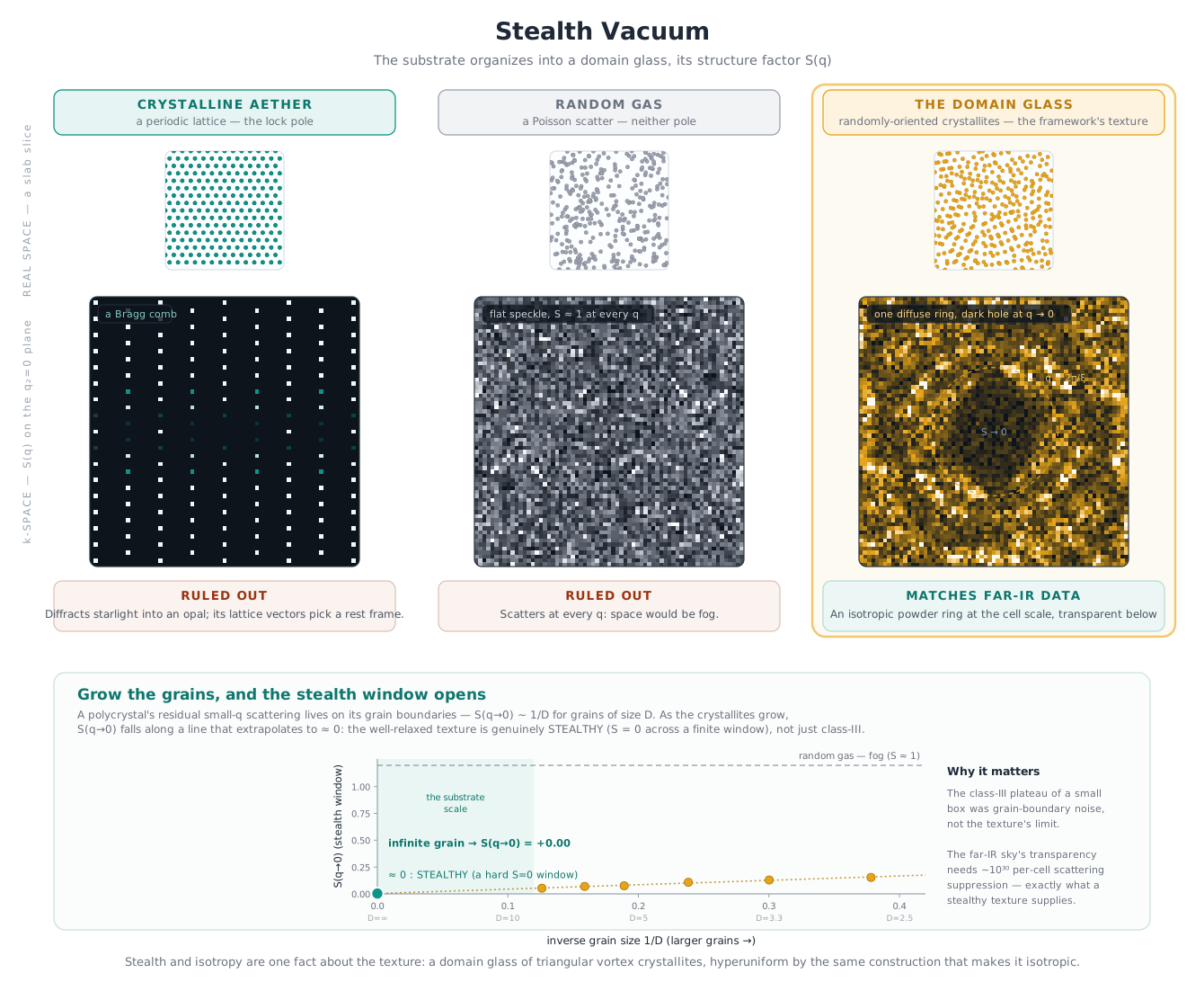
And the data shows that the far-IR sky is transparent until \lambda>2\xi\approx200\,\mum, then begins a faint scattering edge that rises to the ring at \lambda=\xi (\sim3 THz), matching the domain-glass texture, another observation that points to the scale of the lattice.

The same stealth answers an obvious question about gravity. A \sim100\,\mum superfluid lattice filling space sits squarely inside the sub-mm window that Eöt-Wash torsion balances have swept for deviations from Newtonian gravity (roughly 40\,\mum to 11 mm) — yet they see none. The cell scale does not present itself to laboratory masses as an extra gravitational structure: its cross-coupling to ordinary matter is f_\mathrm{cross}\sim10^{-15}, some ten-plus orders of magnitude below torsion-balance sensitivity, so there is no oscillatory sub-mm force to find. The same universal weakness banks the equivalence-principle tests — one gravitational channel, common to all matter, produces no composition-dependent force — consistent with MICROSCOPE’s \eta\lesssim10^{-15}. The one macroscopic scale above the cell — the coherence ceiling \ell_L\approx3.9 cm (§5.7) — is a smoothness null for the same reason, not a signal.

5.5 Two cosmic tensions find a fit

The Hubble and S_8 tensions are both reduced here by the model of the previous cycle’s moraine crust. Fit to the combined DESI DR2 BAO and Jia et al. H_0(z) measurements, the substrate’s one-parameter physical shockwave-envelope density profile reaches a \chi^2\approx42.2, against \LambdaCDM’s \approx821, and suppresses structure growth to S_8=0.816 compared to Planck 2018’s 0.832. Refining the shockwave envelope with the Hubble-tension-reducing freeform 14-knot spline gives S_8=0.807; and factoring in remnant debris in the moraine crust with a Poisson distribution lowers it another |\Delta S_8|\lesssim0.005–0.01, onto the edge of the lensing measurements of 0.76–0.79. Once dark-energy density is allowed to fluctuate, either tension can be reduced by various moraine-crust models; the one that I found that reduces both is the predicted chirping undular bore with a transcritical point at z=1.588, hitting remnants of the last cycle, an essential event in a substrate that nucleates on a periodic cycle.

Figure 16: One moraine-crust profile reduces both tensions. The same density profile fits the joint DESI DR2 BAO + Jia et al. H_0(z) observations, and also reduces the tension with structure growth. Scorecard: \chi^2 for the freeform 14-knot spline, the one-parameter physical shockwave envelope, and the standard model \LambdaCDM. Both substrate fits land just above the weak-lensing window — the freeform spline at S_8\approx0.807 and the shockwave envelope at S_8\approx0.816 — closer than \LambdaCDM’s 0.831

5.6 Tier 2 — physics re-derived

This section has accurately measured physics with a substrate spin. This helps show the substrate model’s consistency and in some cases sharpen the observation, like the W/Z mass ratio to 0.5\%, and frame-dragging, (g-2)/2=\alpha/2\pi.

• The Bohm quantum potential (§1);
• The hydrogen Rydberg spectrum from pilot-wave standing-wave matching³⁸
• Entanglement and Bell’s E(\theta)=-\cos\theta, CHSH 2\sqrt2 — from a twist wave on the vortex channel joining the split pair³⁹
• The Born rule for a spin projection, \cos^2(\theta/2) — the single-quantum Malus law — from the reactive gear-reduction of the counter-rotating boundary layer as the analyzer axis tilts⁴⁰
• The Aharonov–Bohm phase e\Phi/\hbar — real and topological, because the vector potential is the substrate’s co-rotating flow the charge swims in, not a bookkeeping device, so a charge circling shielded flux picks up its enclosed circulation even where the field vanishes⁴¹
• The Sagnac phase \Delta\varphi=\tfrac{2m}{\hbar}\vec\Omega\cdot\vec A — a rotation imprints the enclosed substrate circulation and the matter-wave fringe count is the number of circulation quanta h/m threading the loop, the frame-dragging term read for a laboratory apparatus rather than a gravitating mass⁴²
• The Casimir force -\pi^2\hbar c/240\,d^4 comes from a boundary-shaped modon pressure, a rearrangement of the vacuum’s field, not its energy, with no zero-point sea, per Schwinger/Jaffe, exact where measured (10 nm–μm)
• Vacuum magnetic birefringence \Delta n\propto B^2 shows that field-aligned dc1 flow is the optic axis and the modon’s splitting is the phase delay with the field’s own flow as the lattice rows. Reproduces the Euler–Heisenberg form and scale (B/B_c)^2; magnetar RX J1856 (Mignani 2016), PVLAS bound.
• The electron g=2 and the anomalous moment⁴³
• (g-2)/2=\alpha/2\pi; quark charges +\tfrac23,-\tfrac13 from junction solid angle and \sim99\% of the proton mass from boundary-layer energy (matching lattice QCD)⁴⁴
• The quantum Hall effects — fractional charge e/3 as a Laughlin vortex’s winding fraction (the same charge-as-winding ontology as the quark \tfrac13, here measured directly by shot noise), integer quantization \sigma_{xy}=\nu e^2/h from topological protection of quantized circulation (exact to <10^{-9}, the resistance standard), and the odd/even-denominator rule as the boundary-parity fermion/boson split — even denominators the paired breath at \nu=\tfrac52⁴⁵
• The W/Z mass ratio M_W/M_Z=\cos\theta_W — the standard gauge relation, but as the equatorial spin velocity \beta_\mathrm{eq} of the counter-rotating boundary shell: \cos\theta_W=0.877 against the measured 80.4/91.2=0.882 (0.5\%)⁴⁶
• The CKM-small / PMNS-large mixing asymmetry — quark mixing is small and lepton mixing is large because a mixing matrix is the relative rotation of two \mathbb{Z}_3 generation clocks: up- and down-type quarks are color-loaded to the same side of the generation lock (co-aligned \to small CKM), while charged leptons and neutrinos straddle it (anti-aligned \to large PMNS); the atmospheric angle sits at the pairing-\sqrt2 tilt, \theta_{23}\approx45° (\cos45°=1/\sqrt2), and a large CP-violating Dirac phase is generic in both sectors as the imaginary part of the complex clock \omega=e^{2\pi i/3} — the sign of the asymmetry and near-maximal \theta_{23} reproduced, the individual angles and the CP value still owed⁴⁷
• The Schwarzschild metric and classical GR tests (§3.1)
• Frame-dragging (Lense–Thirring) at the Gravity Probe B rate — the entrained azimuthal component of the same gravitational leak-inflow, v_\phi=2GJ\sin\theta/(c^2r^2) (§4.3): geodetic 6604 vs GP-B 6601.8\pm18.3, frame-drag \approx41 vs 37.2\pm7.2 mas/yr
• Gravity waves travel at the speed of light: c_\mathrm{GW}=c
• Rest energy E=mc^2 (§1.1.1) — the flywheel energy of the internal vortex, \tfrac12m_\mathrm{eff}v_\mathrm{rot}^2 with the rim locked at v_\mathrm{rot}^2=2\alpha_{mf}c^2, with an aperture \alpha_{mf} that decides how much leaks out and is weighable; the \tfrac12 and the 2 cancel and m_ec^2 is what remains, with c derived (Equation 5) and \alpha_{mf}=\tan^2\theta_W fixed, so nothing is left free to choose
• Special relativity — time dilation \gamma, length contraction, and E=\gamma mc^2 — from a moving light-clock: the electron’s internal Compton breath runs on c-bounded substrate signals, so a moving clock slows by the transverse-light-clock factor \gamma=1/\sqrt{1-v^2/c^2} and the de Broglie wave is that same clock seen sideways, unifying the Michelson–Morley null with the pilot wave (exact, zero-parameter)⁴⁸
• The baryonic Tully–Fisher law M_b\propto v^4⁴⁹
• Kleiber’s metabolic law B\propto M^{3/4} from the same boundary-leakage theorem read on a branching vascular network⁵⁰
• The inflationary spectral index n_s\approx0.968 from a sound-speed phase transition⁵¹
• The cosmological constant (§3.2)
• The nuclear binding curve showing iron as the peak.⁵²
• Mass defect ⟷ EMC effect. Mass is a boundary leak, not a bulk count, so binding merges two counter-rotating boundaries into one internal seam — dropping the leaked ledger (the mass defect) and reshaping the reactive ledger (in-medium quark structure, quenched moments/g_A). The sign and universality of the defect are structural, following from a total of -E_\text{bind}/c^2 (which both frameworks match), with EMC strength \propto binding per nucleon.
• Superconductivity’s Cooper pair as the substrate’s anti-phase breath made macroscopic — two same-chirality electrons \pi out of phase in their Compton breathing, one contracted while the other expands, bound by the shared counter-rotating vortex between them (the BCS singlet ↑↓ read as opposite phase, not spin), the charged twin of superfluid ^3He and the lab realization of the very +\omega/-\omega sheet pair the substrate is built from (§4.1)⁵³
• The Hawking temperature T_H=\hbar c^3/8\pi GM, exact — the sonic horizon of the same Painlevé–Gullstrand inflow (§3.1), with 8\pi=2\times4\pi_\mathrm{SC2} the gravitational normalization shared with the Higgs VEV⁵⁴
• The black-hole entropy area law S_\mathrm{BH}=A/4\ell_\mathrm{Pl}^2 — entropy as boundary-crossing leak counted on the one-way horizon seam, hence area not volume⁵⁵
• Neutron stars show the substrate’s vortex unpinning and mutual friction in the context of a neutron superfluid, using the HVBK/\alpha_{mf} boundary coupling match the standard glitch model with recovery set by mutual friction. A canonical 1.4\,M_\odot, 12-km star has a surface that sits at r/r_s\approx3, so the substrate inflow there is v_\text{ebb}=c\sqrt{r_s/R}\approx0.6\,c — the framework’s counter-rotating boundary skin at more than half the signal speed and still closing the seam that keeps matter matter. The dipole is the geodynamo, the canonical loop scaled a billionfold. The pulsar/magnetar split shows a consistent birth and evolution pattern where the rotational budget is partitioned between a coherent-jet channel (the beamed spin-down) and a stored-field channel (released in bursts and giant flares). The glitches are mutual friction (\alpha_{mf}) in that superfluid. The Crab and Vela wind nebulae are the canonical disk–jet–counterflow loop photographed and the pulsar\tomagnetar sequence is a B/B_c ladder of natural birefringence laboratories climbing from \sim0.3\,B_c to \sim45\,B_c. The story holds together even without new numbers.
• The baryon asymmetry \eta_B\approx\varepsilon_\mathrm{chirality}^9=5.8\times10^{-10} † — all three Sakharov conditions native to the boil, the chiral-vacuum bias frozen across nine junction interfaces; the ninth-power exponent is read off the data as a bet, not derived, so it carries the same open-factor dagger as the Tier-1 rows above⁵⁶
• The sonoluminescence flash width stays wavelength-independent into the far-UV / soft X-ray as the substrate predicts. It comes from the bubble’s boundary collapse, from a max R_\text{max}\approx 40–50\;\mum, one half of the lattice cell size, to R_\text{min}\approx 0.5\;\mum at supersonic speeds. The same process that emits a spectral line when an atom’s boundary collapses here causes a stream of photon/modons spread evenly across the spectrum, without an orbital boundary to form the sharp line. Noble gases allow the substrate’s pure energy to be released as modons. Other atoms absorb energy that disrupts the flash effect explaining this poorly understood phenomenon.
• The vacuum itself is a time-crystal formed from the anti-phase \omega_1 breathing. It is hidden in time, the way the lattice is hidden in space, beating a half-cycle out of step, summing to zero above one cell. Lab time crystals surface the vacuum’s breath through chemistry.

5.7 Live predictions — testable now

Between the re-derivations above and the wider net below sit a few concrete numbers (or sharp qualitative breaks) the framework forecasts that have not yet been measured. These are among its best chances to be falsified.

Prediction	Value	Test / instrument
Lightest neutrino mass	m_{\nu,1}\approx m_1\approx2 meV; normal ordering; \Sigma m_\nu\approx61 meV57	DESI+CMB \Sigma m_\nu (\lesssim70 meV), JUNO/DUNE ordering, KATRIN
Gravitational-wave echoes	post-ringdown echoes spaced \sim(r_s/c)\ln(\cdot) from a physical stiff near-horizon shell58	LIGO/Virgo/KAGRA ringdowns, Einstein Telescope, LISA
Coherence-lifetime ladder	persistence climbs by 1/\alpha_{mf}\approx3.32 per balanced wrapping shell; log-lifetime rungs spaced \ln(1/\alpha_{mf})\approx1.2059	qubit T_2 catalogues, time-crystal protection-depth series, mark-erasure timescales, stamp ring-down
GUT-scale Weinberg angle	\sin^2\theta_W\to0 at high energy, against the Standard Model’s \to3/8 — same downward running at accessible scales, opposite endpoint above the TeV60	beyond-TeV collider running, precision electroweak fits
Second substrate scale — a null	coherence ceiling \ell_L=(\nu/4\pi)^{1/3}\xi\approx3.9 cm: forbids sharp coherent substrate structure beyond a few cm and predicts no signal there61	mm–cm torsion balances, mK/microwave searches — a smoothness ceiling, thermally swamped, f_\mathrm{cross}\sim10^{-15}

5.8 Tier 3 — the wider net

Tier 3 includes predictions that suggest the broader pattern. The truth is, if the substrate exists, the biggest question is: how come we can’t see it? And given its ability to hide, it will take a broader lens to find the patterns. I found the substrate by following the broader patterns. It’s the organizational energy between boundary layers at all scales, and so this investigation expands the lens to include the clearest examples of a deeper investigation online.

These are pattern matches, not derived proofs, intended to suggest avenues of future research into how the substrate may act as a hidden organizing layer.

The breadth of these observations invites the objection that they are coincidences. There’s no eliminating that risk, but they are the patterns the same backbone leads you to expect, and each one is another lens on a substrate that is pervasive and yet hides well. The constants are fixed once — K=j_{11}^2+1, the pairing \sqrt2, \alpha_{mf}=\tan^2\theta_W, the condensation number \nu, the rotation speed 0.776\,c, and v_L — and then, with no additional parameters, they make predictions across all of these scales. The backbone and the atomic predictions are accurate where the number of chemistry layers is zero; as you add layers, the crisp numbers get harder to find. But the pattern, the scale, the ratios, and the energy balance show up again and again — all from the backbone’s canonical lengths and ratios, fenced in from cosmology, the electroweak scale, molecular geometry, and the far-IR sky. I found it by triangulating from all sides, and that may be the only way to see it.

With more substrate layers, the Tier 3 predictions are more qualitative than quantitative. The quantitative matches could individually be a coincidence, the ratio and scale found here and there, but the pattern that keeps surfacing between scales and domains is an important part of the puzzle. The same constants reappear as you would expect them to supported by the backbone. The same patterns organize boundary layers at all scales.

The substrate has a signature, regardless of the material. It locks onto the \sqrt2 size-comb and its octave when parts need to nest and trade energy; it anti-locks onto the golden gap \varphi when they need to stay independent, wearing whichever face the space allows — 137.5^\circ on a circle, disordered-hyperuniform blue noise on a plane, coprime or \varphi-spaced periods in time; it minimizes the one counter-rotating boundary energy \tfrac12\rho(\Delta v)^2 at every scale; it sheds excess spin through a single disk–jet–counterflow loop; and it marks a few characteristic speeds (v_L\approx750 km/s, its own rotation 0.776\,c). So the wider net is best read as one substrate signing its name with the same handful of marks in domains that have no business sharing a constant — the same \sqrt2, \varphi, and \tfrac12\rho(\Delta v)^2 placing a quark, a leaf, a cone cell, and a musical interval.

• Grid cells step by \sim1.4\approx\sqrt2 — the bare ladder rung — across species.
• Phyllotaxis sets each leaf at the golden angle 137.5^\circ (\varphi on a circle), realized by the same flux-lattice physics the substrate is built from (Levitov 1991), magnet-free.
• The retinal cone mosaic tiles as disordered hyperuniform blue noise — the planar face of choosing anti-lock in the substrate ladder. This avoids image aliasing.
• The same sealed d^{10} boundary smoothness that makes copper, silver and gold the best normal conductors forbids them from superconducting, while rough-shelled niobium, vanadium and tantalum pair readily — T_c anti-correlates with inner-boundary smoothness across the transition metals.⁶²
• The outer rim onset speed v_L=\omega_0\xi \approx750 km/s surfaces as a boundary gating the galactic MOND→CDM transition and near the peak of the Sun’s fast polar wind (Ulysses mean 751.5 km/s).
• The inner-rim \gamma shoulder shows that an electron driven to the substrate’s own rotation speed (0.776\,c) tears its boundary and sheds a \sim300 keV gamma modon; the electron–electron bremsstrahlung shoulder at T_e\approx300 keV — a 200–500 keV excess over combined bremsstrahlung, with a fatter angular distribution — in terrestrial \gamma-ray flashes (TGF/ALOFT), solar flares (RHESSI/STIX/NuSTAR), and tokamak hard-X-ray disruptions.
• Cell sorting is boundary-energy minimization one rung up: an embryonic tissue behaves as an immiscible liquid whose measured surface tension is the same counter-rotating-layer energy \tfrac12\rho_\text{cr}(\Delta v)^2 read at the cell cortex, with cadherins setting the velocity match — and the sorting topology is a dressing-cancelled tension ratio the data already bear out (transitive hierarchies, an E-cadherin phase reversal, a vanishing adhesion-bond term), the same knob whose pathological failure is metastasis.⁶³
• Twelve-tone equal temperament fills the octave with twelve steps of 2^{1/12}, so the tritone lands at 2^{6/12}=\sqrt2 exactly — the substrate’s bare half-octave hinge — while the octave (2{:}1) and the fifth (3{:}2) sit on the comb’s cleanest teeth. Music theory has always heard the difference: the consonances are locks, and the tritone on the hinge is the diabolus in musica — the same \sqrt2 that half-registers two lattice sheets, now something anyone can hear.
• Cortical rhythms play both ends of the ladder in time: when it binds, the cortex nests its bands at octaves (integer theta–gamma phase-locking); at rest it spreads them to a non-locking irrational near the half-octave so they coexist without interference — either the substrate’s \sqrt2 or the most-irrational \varphi\approx1.618 the resting-EEG literature reports (Pletzer et al. 2010), a live {\sim}14\% test that either way is one gap read on the time axis.
• The solar system writes lock and anti-lock across the sky at once: the Galilean moons hold a 1{:}2{:}4 Laplace chain — an octave stacked twice, the cleanest tooth there is — and Neptune and Pluto ride a protected 3{:}2, bodies locking onto the comb; while the Kirkwood gaps in the asteroid belt are swept clean at the integer resonances, the survivors fleeing the tooth. One ladder, two ends, in orbits.
• Earth’s mantle runs the disk–jet–counterflow loop one rung up from a black hole: whole-mantle convection organizes into a degree-2 pattern with two roughly antipodal superplume feet — the African “Tuzo” and Pacific “Jason” LLSVPs, each {\sim}10{,}000 km across — as the counter-rotating dipole cores, wrapped by the {\sim}200 km D'' layer at the core–mantle boundary as the enclosing sheath. The same feedback topology that shapes an accreting spinner, at planetary scale.
• The Earth’s crust shows both substrate poles in rock. A major fault locks along some stretches — its rough walls nested in register, storing elastic strain for centuries, then spending it all at once as an earthquake — and creeps along others, the walls refusing to catch, sliding a few millimetres a year and never building toward rupture; the San Andreas and the Hayward do both at once, along their length and down their depth. The same lock/anti-lock split reads a cookie’s clean snap (a brittle lattice failing along its cheapest pre-existing seam — exactly how a fault nucleates), the six-fold basalt column (locked, in register), and a road-cut’s two joint sets meeting at right angles in junctions that refuse to merge (anti-lock). Other domains show both poles too, but by state or by orbit; the crust is where they share a single fault, outcrop, and hand specimen — the ladder (§4.2) made not just visible but touchable.
• Sonoluminescence is the lightning \gamma-shoulder’s twin at a wildly different scale: the line-free picosecond flash from a collapsing bubble is a boundary driven to reverse past the substrate’s own rotation speed 0.776\,c, tearing and shedding a modon — except here the boundary is macroscopic, the collapsing gas–liquid interface itself rather than an electron’s coherence dress.
• Helium-3, the one atom cold enough to mirror the substrate, carries the pairing-two in the open: it must first assemble an anti-phase paired boson before it can lock to the vacuum’s breath, so it goes superfluid only {\sim}1000\times colder than He-4 ({\sim}1 mK versus {\sim}2 K) and stamps the factor of two directly into its circulation quantum h/2m_3 — the same pairing-two the framework meets everywhere it probes the lattice.

5.8.1 Molecular recognition — one stamp metric, many reads

At the cellular scale, the substrate’s energy gets wrapped into nested layers of chemistry. But these nested layers make it hard for direct measurements to differentiate the substrate’s energy from what we already model through chemistry.

At the cellular scale, the numbers you’d expect to match do seem to match.

An aromatic ring shows clearly as a toroidal vortex — the closed surface that earns benzene its {\sim}36 kcal/mol of aromatic stabilization, a closed-loop flow with no ribbon end to terminate.⁶⁴ Each nucleobase is then a stack of one or two such tori, and a codon, a base pair, or a binding pocket is a three-dimensional stamp: the superposition of those per-base vortex profiles on the substrate’s flow geometry. One set of per-base profiles, one overall scale, no per-observable tuning, feeds an L^2 overlap metric that reads out across three independent classes of molecular recognition. No single row below is a paper-central number — but as a group they put numeric weight under the cellular-dynamics chapters: the same metric that places every cognate anticodon first also tracks drug-binding affinity across four orders of magnitude and beats additive hydrogen-bond counting on base-pair stability.

Observable	Substrate reading	Result
Benzene aromatic stabilization	closed-torus π flow, no edge to terminate65	{\sim}36 kcal/mol — matches
G:C / A:T pair stability	per-lobe vortex overlap, non-additive66	ratio 1.69 (measured 1.8–2.0; additive H-bonds give 1.5)
Codon–anticodon cognate recognition	64\times64 stamp-overlap matrix67	cognate ranks #1 for 64 of 64
Synonymous vs non-synonymous spread	same metric, no retuning68	stamp-distance ratio 1.75
nAChR agonist affinity	aromatic-pocket stamp distance69	Spearman \rho=+0.905 vs measured K_i
5mC reader split	major-groove stamp-edit, WC face intact70	groove readers respond, WC-edge readers blind (retrodiction, holds)
Olfactory OR repertoire	anti-lock pole in stamp space	hyperuniform, not Poisson ({\sim}400 pockets, untested)

Each row supports the overall point — that substrate energy influences and organizes cellular dynamics, offering a hidden information channel mediated by chemistry.

See more at https://lightfluid.org/predictions.html.

6 Reproducing the numbers

Most numerical predictions are demonstrated by three python scripts:

python3 scripts/substrate_atomic.py     # particle-physics backbone + lattice
python3 scripts/substrate_gravity.py    # gravity sector
python3 scripts/substrate_galactic.py   # DESI / Hubble cosmology

7 Open problems

• The 4\pi in SC2 and in the bridge equation’s geometric value and the following results rely on the substrate’s emergent Lorentz invariance being exact, supported by observation but not derived. The induced (Einstein–Hilbert) action gives the equation the 4\pi automatically once that is shown. It is also supported by Michelson–Morley and GW170817.

• The nonlinear completion of the Einstein equations requires a formal proof.

• For dark matter, the quantitative step from the Hubble flow’s DC parity-bias to the coefficient of a_0=c\sqrt{G\rho_\mathrm{DM}} (§3.3) — equivalently, a phonon-mediated force profile reproducing the full radial-acceleration relation at galactic scales — is still open.

• Finding the nuclear surface scale profile a_S. Only the iron-peak has been predicted so far.

• Derive the nuclear coupling \alpha_{mf}^{(N)}\approx552 (§1.1) independently — from nuclear-scale vortex packing, the way \tan^2\theta_W fixes the electronic \alpha_{mf}^{(e)}=0.3008. At present \alpha_{mf}^{(N)} is back-solved from the measured proton mass through the shared quantum m_\mathrm{eff}, so the proton-to-electron mass ratio is a re-parametrization rather than a prediction; an independent count \sim552 would turn m_p/m_e\approx1836 into a genuine output.

• Derive the condensation number \nu=m_\mathrm{eff}/m_1=8.35\times10^8 (Equation 12). It is now over-determined — cosmology \times the geometric cell occupancy, the measured Higgs VEV, and the fast solar wind all land on it, the first two to 0.12\% — but no bottom-up calculation produces it from first principles. It is the framework’s single sharpest open number: the lattice size, the Higgs VEV, v_L, and the MOND scale all ride on it.

• Show the substrate ladder’s properties support scale invariant properties.

• Formal proof of the lattice spacing from the logarithmic equation of state’s maximum packing result.

Conclusion

I am not an expert in any of the domains this paper covers but have been avidly reading science papers for a long time. You may see something I missed, but to me, this feels like a worthy direction to pursue, and I welcome any help to improve it.

In 1861 Maxwell built his theory of electromagnetism on molecular vortices, and six years later Thomson proposed the vortex atom. Neither had the superfluid model needed to account for inertia or the electron’s orbit, and they moved on.

Volovik found key properties of the universe in a supercooled droplet of He-3, the one atom that stays fluid cold enough to tune into the anti-phase breathing of the substrate, and so essentially a mirror of the substrate itself. Bush, Zloshchastiev, Khoury, and many others supplied more pieces of the puzzle.

Treating Madelung/Bohm and Simeonov’s fluid as a superfluid, the quantum potential becomes the reaction force of the boundary layer. The photon makes perfect sense as a modon — wrapping up these counter-spinning layers and using the substrate’s energy to launch itself. Once Planck’s constant, light’s minimum packet size, is used as the modon’s minimum size, the lattice size is fixed and these predictions follow. The behavior of superfluids unifies science behind one physics — without strange assumptions.

The stealthy superfluid turns quantum uncertainty into a measurement artifact. Entanglement is explained by the split pair’s topologically protected vortex lines, which still join them across long distances. When you measure one end, a twist wave runs back down that cleared, laminar channel faster than the speed of light, reproducing the Bell correlations (§5.6). The unique properties of the superfluid — its stiff local behavior, cold distant appearance, and its phase transitions — explain gravitational lensing and time dilation as pressure effects, not strange physics.

To me, Our Big Bubble and Our Fluid Universe make more sense. When reading Bush’s paper, I had the realization that the photon is a modon. It did not take long to find the math, but it took time to accept the large size of the lattice, and to see how the energy flows create a common topology — the orbital plane, the polar jets, the modon topology that holds the energy. Given the sheet spacing, that leads to the ladder influencing boundary effects, and to chemistry creating long vectors by organizing against the lock/anti-lock pattern, storing them as coherent substrate layers and transmitting them as complex modons. With hidden organization, information, and energy, the substrate drives cellular dynamics — replacing the hard-to-accept notion that cells run on chaos alone. The Earth evolved by nesting and folding substrate layers to trap substrate energy into persistent modons, and life evolved by folding and trapping more.

The substrate framework offers a new lens to help uncover the nature of the superfluid that underlies everything, and its hidden lattice.

Find a deeper investigation at https://lightfluid.org.

Acknowledgements

This paper was made possible by the work of many scientists included in the references.

In particular, Volovik, Bush, Oza, Simeonov, Zloshchastiev, Khoury, Larichev and Reznik provided the foundational math and inspiration.

I’m also grateful to my amazing employer Posit PBC, supporters of open source software for data science. This is an unaffiliated side project, and naturally open source.

References

Abo-Shaeer, J. R., C. Raman, J. M. Vogels, and W. Ketterle. 2001. “Observation of vortex lattices in Bose–Einstein condensates.” Science 292: 476–79.

Avdeenkov, A. V., and K. G. Zloshchastiev. 2011. “Quantum Bose liquids with logarithmic nonlinearity: self-sustainability and emergence of spatial extent.” Journal of Physics B: Atomic, Molecular and Optical Physics 44: 195303. https://arxiv.org/abs/1108.0847.

Barceló, C., S. Liberati, and M. Visser. 2005. “Analogue gravity.” Living Reviews in Relativity 8: 12.

Baym, G. 2003. “Tkachenko modes of vortex lattices in rapidly rotating Bose–Einstein condensates.” https://arxiv.org/abs/cond-mat/0305294.

Bekarevich, I. L., and I. M. Khalatnikov. 1961. “Phenomenological derivation of the equations of vortex motion in He II.” Soviet Physics JETP 13: 643–46.

Berezhiani, L., and J. Khoury. 2015. “Theory of dark matter superfluidity.” Physical Review D 92: 103510.

Bezdek, A., and W. Kuperberg. 1990. “Maximum density space packing with congruent circular cylinders of infinite length.” Mathematika 37 (1): 74–80. https://doi.org/10.1112/S0025579300012808.

Bialynicki-Birula, I., and J. Mycielski. 1976. “Nonlinear wave mechanics.” Annals of Physics 100: 62–93.

Braaten, E., and H.-W. Hammer. 2006. “Universality in few-body systems with large scattering length.” Physics Reports 428: 259–390.

Bush, J. W. M., and A. U. Oza. 2020. “Hydrodynamic quantum analogs.” Annual Review of Fluid Mechanics 52: 235–80.

Donnelly, R. J. 1991. Quantized Vortices in Helium II. Cambridge University Press.

Ennola, V. 1964. “A lemma about the Epstein zeta-function.” Proceedings of the Glasgow Mathematical Association 6 (4): 198–201. https://doi.org/10.1017/S2040618500034961.

Fetter, A. L. 2009. “Rotating trapped Bose–Einstein condensates.” Reviews of Modern Physics 81: 647.

Glaberson, W. I., W. W. Johnson, and R. M. Ostermeier. 1974. “Instability of a vortex array in He II.” Physical Review Letters 33: 1197.

Goles, E., O. Schulz, and M. Markus. 2001. “Prime number selection of cycles in a predator–prey model.” Complexity 6 (4): 33–38.

Hall, H. E., and W. F. Vinen. 1956. “The rotation of liquid helium II. II. The theory of mutual friction in uniformly rotating helium II.” Proceedings of the Royal Society A 238: 215–34.

Hamilton, A. J. S., and J. P. Lisle. 2008. “The river model of black holes.” American Journal of Physics 76: 519.

Jiménez, J. 1975. “Stability of a pair of co-rotating vortices.” Physics of Fluids 18: 1580–81.

Khoury, J. 2015. “A dark matter superfluid.” https://arxiv.org/abs/1507.03013.

Larichev, V. D., and G. M. Reznik. 1976. “Two-dimensional solitary Rossby waves.” Doklady Akademii Nauk SSSR 231: 1077–79.

Levitov, L. S. 1991. “Phyllotaxis of flux lattices in layered superconductors.” Physical Review Letters 66: 224.

McGaugh, S. S., F. Lelli, and J. M. Schombert. 2016. “Radial acceleration relation in rotationally supported galaxies.” Physical Review Letters 117: 201101.

Mehdi, Z., J. J. Hope, S. S. Szigeti, and A. S. Bradley. 2023. “Mutual friction and diffusion of two-dimensional quantum vortices.” Physical Review Research 5: 013184. https://arxiv.org/abs/2205.04065.

Moffatt, H. K. 1969. “The degree of knottedness of tangled vortex lines.” Journal of Fluid Mechanics 35: 117–29.

Planck Collaboration, N. Aghanim, et al. 2020. “Planck 2018 results. VI. Cosmological parameters.” Astronomy & Astrophysics 641: A6. https://arxiv.org/abs/1807.06209.

Rankin, R. A. 1953. “A minimum problem for the Epstein zeta-function.” Proceedings of the Glasgow Mathematical Association 1 (4): 149–58. https://doi.org/10.1017/S2040618500035668.

Reznik, G. M. 2010. “Dynamics of localized vortices on the beta plane.” Izvestiya, Atmospheric and Oceanic Physics 46 (6): 784–97. https://doi.org/10.1134/S0001433810060095.

Rosen, N. 1968. “Dynamics of a particle as a solution of a nonlinear field theory.” Journal of Mathematical Physics 9: 996.

Saffman, P. G. 1992. Vortex Dynamics. Cambridge University Press.

Sakharov, A. D. 1967. “Vacuum quantum fluctuations in curved space and the theory of gravitation.” Doklady Akademii Nauk SSSR 177: 70–71.

Sandier, E., and S. Serfaty. 2012. “From the Ginzburg–Landau model to vortex lattice problems.” Communications in Mathematical Physics 313 (3): 635–743. https://doi.org/10.1007/s00220-012-1508-x.

Simeonov, L. 2025. “Quantum potential from the material derivative of the osmotic velocity: a two-fluid Madelung framework.” https://arxiv.org/abs/2509.02868.

Sornette, D. 1998. “Discrete scale invariance and complex dimensions.” Physics Reports 297: 239–70.

Stensola, H., T. Stensola, T. Solstad, K. Frøland, M.-B. Moser, and E. I. Moser. 2012. “The entorhinal grid map is discretized.” Nature 492: 72–78.

Tkachenko, V. K. 1966. “On vortex lattices.” Soviet Physics JETP 22: 1282.

Unruh, W. G. 1981. “Experimental black-hole evaporation?” Physical Review Letters 46: 1351.

Volovik, G. E. 2003. The Universe in a Helium Droplet. Oxford University Press.

Zloshchastiev, K. G. 2020. “Superfluid vacuum theory and deformed dispersion relations.” International Journal of Modern Physics A 35: 2040032.

Footnotes

1. Originally named with the idea that dark carbon buckyballs (e.g. dc60) might help in modeling elastic collisions or compression in black holes. Thankfully, a single elastic, nucleating substrate particle saves us from all of that. And although dc1 is also seen as dark matter, it’s important to see that the substrate underlies everything: protons, electrons, and other particles are topologically protected vortices and knots, orbital systems.

2. Simeonov’s derivation (Simeonov 2025) takes a single fluid of density \rho obeying the diffusion law \mathbf J=-D\nabla\rho; its velocity is the osmotic velocity \mathbf u=\mathbf J/\rho=-D\nabla\ln\rho. Form its material (convective) derivative — the osmotic acceleration \mathrm d\mathbf u/\mathrm dt=\partial_t\mathbf u+(\mathbf u\cdot\nabla)\mathbf u — and substitute the continuity equation \partial_t\rho=-\nabla\!\cdot\mathbf J=D\nabla^2\rho for the time part. The time and convective pieces collapse into a single gradient, \mathrm d\mathbf u/\mathrm dt=\nabla\!\left(-2D^2\,\nabla^2\!\sqrt{\rho}/\sqrt{\rho}\right), whose bracket is the Bohm quantum potential per unit mass, Q/m, the instant one sets D=\hbar/2m (then 2D^2=\hbar^2/2m^2 and Q=-\frac{\hbar^2}{2m}\,\nabla^2\!\sqrt{\rho}/\sqrt{\rho}). So Q is the inertia of the osmotic flow, and the convective term (\mathbf u\cdot\nabla)\mathbf u is what produces it. To turn this identity into a force on a physical density, Simeonov uses two fluids: fluid 2 mutually diffuses down fluid 1’s gradient, \mathbf J_2=-D\nabla\rho_1, and is re-equalised to it on a fast timescale, so its osmotic acceleration is the expression above with \rho\to\rho_1; by Newton’s third law its reaction on fluid 1 is exactly \mathbf F_\mathrm{reaction}=-\nabla Q (Equation 2). Fed into fluid 1’s Euler equation beside an ordinary potential U, this returns the full Madelung system — hence, through \Psi=\sqrt{\rho_1}\,e^{iS/\hbar}, the Schrödinger equation; a relativistic diffusion law J^\mu=D\,\partial^\mu\rho runs the identical steps to Klein–Gordon. For Step 1 the framework reads fluid 1 as the co-rotating dc1 bulk and fluid 2 as a counter-rotating HVBK boundary layer, so that his diffusion constant becomes the circulation-set diffusivity D_{sf}=\kappa_q/(4\pi\alpha_{mf}) of §1.1 and Simeonov’s fast density-equalising “jumps” become the boundary layer continuously re-tracking the bulk gradient. The quantum potential and \hbar=2mD are then a single statement read at two levels: Simeonov’s kinematics, and the substrate’s hydrodynamics.

3. Here \kappa_q/4\pi is the standard local-induction self-velocity coefficient of a quantized vortex filament (Saffman 1992; Donnelly 1991), \kappa_q = h/m_\mathrm{eff} the Onsager–Feynman circulation quantum, and \alpha_{mf} the HVBK mutual-friction coupling (Hall and Vinen 1956; Bekarevich and Khalatnikov 1961). The expression is a dimensional identification of the friction-limited transport scale — its content is the scaling D_{sf}\propto\kappa_q/\alpha_{mf} with the 4\pi local-induction prefactor — not a quoted closed-form coefficient. (The distinct thermal vortex-diffusion coefficient has the Einstein form D\propto\alpha_{mf}\,k_BT (Mehdi et al. 2023); what enters here is the athermal, circulation-set transport scale.)

4. The value \alpha_{mf}=0.3008 comes from the Weinberg angle using a friction ratio equation. The HVBK mutual-friction force has two pieces: a reactive part (deflection that turns the flow’s chirality without transferring energy) and a dissipative part (drag that carries energy across the boundary). Identifying the reactive channel with the SU(2)_L weak coupling g and the dissipative channel with the U(1)_Y hypercharge coupling g' makes the friction ratio the coupling ratio, \alpha_{mf}=\frac{g'^2}{g^2}=\tan^2\theta_W,\qquad\text{equivalently}\qquad \sin^2\theta_W=\frac{\alpha_{mf}}{1+\alpha_{mf}}, so the measured \sin^2\theta_W=0.2312 fixes \alpha_{mf}=0.2312/0.7688=0.3008. This sits squarely in the range real two-fluid superfluids show in their active regime (He-II passes \alpha\approx0.3 near T/T_\lambda\approx0.6): \approx30\% of each boundary interaction dissipates, \approx70\% deflects. The same parameter also represents a vortex-scattering phase, \alpha_{mf}=\tfrac12\sin2\delta_0 with \delta_0=18.48^\circ (the weak-scattering branch, selected by \alpha\ll1) — the geometric input behind the fine-structure-constant and magnetic-moment predictions of §5. Currently \alpha_{mf} comes from a measured input. It might be possible to compute it from the equilibrium spin rate of the counter-rotating boundary.

5. m_\mathrm{eff} is taken to be a property of the substrate, not of the particle it builds — one quantum of dc1 circulation, the same in the electronic and nuclear sectors. Quoting m_e = 0.511\;\mathrm{MeV}/c^2, Equation 3 fixes it once and for all: m_\mathrm{eff} = m_e/\alpha_{mf} = 0.511/0.3008 = 1.70\;\mathrm{MeV}/c^2. Applying Equation 3 in the nuclear sector with this same quantum then defines the proton coupling \alpha_{mf}^{(N)} = m_p/m_\mathrm{eff} = 1836\times0.3008 \approx 552: the proton is \sim552 effective quanta (552\times1.70\;\mathrm{MeV} \approx 938\;\mathrm{MeV} = m_p c^2), while the electron is a 0.3008 fraction of a single quantum. This is a re-parametrization of m_p, not a prediction of it: \alpha_{mf}^{(N)} is back-solved from the measured proton mass, so the identity \alpha_{mf}^{(N)}/\alpha_{mf}^{(e)} = m_p/m_e is algebraic. It would become a genuine prediction only if \alpha_{mf}^{(N)} — equivalently the count \sim552 — could be fixed independently from nuclear-scale vortex packing, the way \tan^2\theta_W fixes the electronic coupling. That derivation is left open (§7).

6. The observation about the spectrum comes from Volovik, The Universe in a Helium Droplet (2003), §7.4.3–7.4.4. The Bogoliubov quasiparticle energy of a pair-correlated fermionic vacuum is E^2 = M^2(\mathbf p) + c^2 p^2 with c=\Delta_0/p_F (his eqn 7.49); in the strong-coupling deep-BEC limit mc^2\gg|\mu| this deforms continuously into the relativistic Dirac form E^2=\mu^2+c^2p^2 (eqn 7.51), with the chemical potential \mu playing the role of the rest mass. The framework’s one added identification is that the dc1 coherence length is the dc1 Compton wavelength, \xi=\hbar/(m_1 c) — equivalently \Delta_0\simeq\mu=m_1c^2 and p_F\simeq\hbar/\xi, so c=\Delta_0/p_F=\hbar/(m_1\xi). This same \xi=\hbar/(m_1c) is the close-packing input of Route 1 (Equation 8). Strong coupling is also what makes the cone isotropic: the spectrum depends on |\mathbf p| alone, so c_\parallel=c_\perp — unlike weak-coupling ^3He-A, whose point-node spectrum is strongly anisotropic (c_\perp/c_\parallel\sim10^{-5}; Volovik §7.4.6). A single isotropic cone shared by every sector is the origin of c_\mathrm{GW}=c.

7. The modon is the Larichev–Reznik two-dimensional Rossby soliton (Larichev and Reznik 1976); its explicit interior/exterior construction and matching are eqns (1.25)–(1.26) of Reznik’s review (Reznik 2010). With the dipole streamfunction \psi=\sin\theta\,J_1(pr) inside and \psi=\sin\theta\,K_1(qr) outside, continuity of \psi and of the normal and tangential velocity at the separatrix r=\xi gives the transcendental matching \dfrac{J_2(p\xi)}{p\,J_1(p\xi)}=-\dfrac{K_2(q\xi)}{q\,K_1(q\xi)} (Reznik eqn 1.26, here in our convention: interior wavenumber p, exterior decay q). The lowest mode lays the first J_1 lobe exactly across one cell, p\xi=j_{11}=3.8317 (the first zero of J_1), with the exterior decaying over one coherence length, q\xi=1. These two — the interior lobe spanning exactly one cell and the exterior tail decaying over exactly one cell — are adopted as the natural mode convention, not read off as an exact root of the transcendental condition above (indeed p\xi=j_{11} makes J_1(p\xi)=0, so it is the sharp-lobe limit of that matching rather than a finite solution of it). The L–R speed denominator is then p^2+q^2=(j_{11}^2+1)/\xi^2\equiv K/\xi^2, which defines K=j_{11}^2+1=15.68. Setting the resulting modon speed equal to c collapses back to the Volovik relation c=\hbar/(m_1\xi) — so modon matching is not a second independent condition but the statement of why a counter-rotating dipole riding the dc1 circulation gradient \kappa_1=2\pi\hbar/m_1 propagates at exactly c. The pair’s vanishing net mass transport — the hydrodynamic content of “massless” — is Reznik’s Property 8, \int\psi\,dx\,dy=0 (eqn 1.18).

8. Two steps. (i) Existence condition 1 fixes the threshold wavelength at one cell, \lambda_\mathrm{min}=\xi (the perturbation envelope has no smooth J_1–K_1 match below \xi). A modon carries photon energy E=h\nu=hc/\lambda, so the one-cell modon has E_\mathrm{min}=hc/\xi. (ii) Substituting \hbar/\xi=m_1c (the Volovik relation, Equation 5) gives the clean identity E_\mathrm{min}=hc/\xi=2\pi(\hbar/\xi)c=2\pi\,m_1c^2: exactly 2\pi times the dc1 rest energy m_1c^2 — the 2\pi is one full circulation loop of the cell (the dc1 circulation quantum being \kappa_1=2\pi\hbar/m_1), m_1c^2 the rest energy of the single dc1 wavefunction per cell. Numerically m_1=m_\mathrm{eff}/\nu=2.03 meV gives E_\mathrm{min}=12.8 meV at \lambda=\xi=97\,\mum, i.e. a crossover frequency c/\xi\approx3.1 THz. This is a floor on a single localized modon — one whose whole counter-rotating dipole fits inside one cell — not a cutoff on the electromagnetic spectrum. Ordinary high-frequency light sits far above threshold (\lambda\ll\xi — visible light is \sim2 eV): it keeps the \xi-scale envelope while concentrating its energy in a compact sub-cell dipole core (the “boat in a harbor,” a compact hull with a basin-wide wake), and at threshold core and envelope coincide at \xi. Below threshold (\lambda>\xi) the dipole can no longer localize inside one cell, and the excitation becomes a delocalized collective modon mode — a coherent, in-phase superposition of the field across many cells, its energy h\nu spread over a region \sim\lambda\gg\xi. This is how light below the floor exists: as the many-cell collective limit of the same modon field, exactly as a long-wavelength acoustic phonon is a single quantum of collective motion whose energy lies far below any one atom’s vibrational quantum. Radio, microwave, and the CMB (peak \sim0.7 meV, a factor \sim20 below threshold) are this collective regime; a single circuit-QED microwave photon (\sim5 GHz, \sim20\,\mueV) is one such collective quantum, its 6-cm wavelength spanning hundreds of cells end to end. So 12.8 meV is a crossover (\lambda=\xi) between a compact single-cell core and a many-cell collective mode, not a spectral edge; any observable would be a change in modon structure and dispersion near 3 THz, not an absence of radiation (§5.2).

9. The elimination proceeds with three steps. Volovik’s speed (Equation 5) gives m_1=\hbar/(c\xi); the composition n_1m_1=\rho_\mathrm{DM} then gives n_1=\rho_\mathrm{DM}\,c\,\xi/\hbar; and close-packing n_1\xi^3=1 gives \rho_\mathrm{DM}\,c\,\xi^4/\hbar=1, i.e. \xi=(\hbar/\rho_\mathrm{DM}c)^{1/4}. The only physical content beyond \hbar,c,\rho_\mathrm{DM} is the quantum-degeneracy condition n\lambda_{dB}^3\sim1 that defines Bose condensation — one coherent wavefunction per de Broglie volume — read here at the lattice cell, \lambda_{dB}\to\xi. Numerically \hbar/(\rho_\mathrm{DM}c) = 1.055\times10^{-34}/(2.254\times10^{-27}\cdot2.998\times10^8) = 1.561\times10^{-16}\,\mathrm{m}^4, whose fourth root is 111.8\,\mum. The “\approx1” is exact only for one wavefunction per cell; the true occupancy is the cell occupancy f (Equation 14), so Route 1 is the f\!=\!1 idealization and the real cell is smaller by f^{1/4}.

10. Planck reports the dimensionless cold-dark-matter density \Omega_c h^2 = 0.1200 \pm 0.0012 (Planck Collaboration et al. 2020); the mass density follows from the critical density, \rho_\mathrm{DM} = \Omega_c h^2 \cdot \rho_\mathrm{crit}/h^2 = 0.1200 \times 1.878\times10^{-26}\;\mathrm{kg/m}^3 = 2.254\times10^{-27}\;\mathrm{kg/m}^3, with \rho_\mathrm{crit}/h^2 = 3H_0^2/(8\pi G h^2) = 1.878\times10^{-26}\;\mathrm{kg/m}^3. The \pm1\% uncertainty on \Omega_c h^2 carries directly to \rho_\mathrm{DM}.

11. The circulation \kappa_q=2\pi\hbar/m_\mathrm{eff} is the ordinary quantum of circulation for a quantum of mass m_\mathrm{eff} (§1.1); the Compton frequency \Omega_v=2m_\mathrm{eff}c^2/\hbar is twice its rest energy over \hbar, the zitterbewegung rate. Explicitly \kappa_q\Omega_v=(2\pi\hbar/m_\mathrm{eff})(2m_\mathrm{eff}c^2/\hbar)=4\pi c^2, with m_\mathrm{eff} cancelling — which is why SC2 is a normalization identity, not a dynamical equation: it fixes which 4\pi the lattice must present in order to gravitate. The field-theory reason that coefficient is precisely the induced-Newton 4\pi — one-loop induced gravity (Seeley–DeWitt) and Jacobson’s horizon thermodynamics both landing the same number — is spelled out in §2.3.

12. The two legs evaluated on the paper’s stated constants: \bar\lambda_\mathrm{eff}=\hbar/(m_\mathrm{eff}c)=116.2 fm with m_\mathrm{eff}=m_e/\alpha_{mf}=1.699 MeV/c^2; the cosmology-plus-geometry cell \xi=\xi_\mathrm{CP}f^{1/4}=111.8\times0.8676=97.0\,\mum gives \nu=97.0\,\mu\mathrm{m}/116.2\,\mathrm{fm}=8.348\times10^8, while \nu=v^2/(8\pi m_\mathrm{eff}^2c^4)=246220^2/(8\pi\cdot1.699^2)=8.358\times10^8. Equivalently m_1=m_\mathrm{eff}/\nu=2.03 meV. The gap between the two is 0.12\% at the Planck central density; it moves between roughly 0.04\% and 0.12\% across the usual roundings of \rho_\mathrm{DM} within Planck’s \pm1\%, which is the honest precision of the comparison. The heliospheric leg, \nu=4\pi(c/v_L)^3=7.98\times10^8, sits 4.4\% low — read the other way, the same \nu predicts v_L=c(4\pi/\nu)^{1/3}=740 km/s against Ulysses’ 751.5 (1.5\%; the cube root divides the discrepancy by three).

13. Equation 14 is the same statement as Route 1 with the “\approx1” made honest: n_1\xi^3=f rather than n_1\xi^3\approx1. Evaluated on the electroweak leg’s cell, \xi=\nu\,\bar\lambda_\mathrm{eff}=97.1\,\mum with \nu from the measured VEV, it returns f=0.5694 against the geometric 0.5666 — a 0.5\% match using the Planck density \rho_\mathrm{DM}=2.254\times10^{-27}\,\mathrm{kg/m}^3. Evaluated on the cosmology-plus-geometry cell it returns 0.5666 identically, because that cell was built from f; the content of the comparison is therefore entirely in the electroweak leg, which is why the pure-number form (the \nu table above) is the statement to quote.

14. The two legs evaluated on the paper’s stated constants: \bar\lambda_\mathrm{eff}=\hbar/(m_\mathrm{eff}c)=116.2 fm with m_\mathrm{eff}=m_e/\alpha_{mf}=1.699 MeV/c^2; the cosmology-plus-geometry cell \xi=\xi_\mathrm{CP}f^{1/4}=111.8\times0.8676=97.0\,\mum gives \nu=97.0\,\mu\mathrm{m}/116.2\,\mathrm{fm}=8.348\times10^8, while \nu=v^2/(8\pi m_\mathrm{eff}^2c^4)=246220^2/(8\pi\cdot1.699^2)=8.358\times10^8. Equivalently m_1=m_\mathrm{eff}/\nu=2.03 meV. The gap between the two is 0.12\% at the Planck central density; it moves between roughly 0.04\% and 0.12\% across the usual roundings of \rho_\mathrm{DM} within Planck’s \pm1\%, which is the honest precision of the comparison. The heliospheric leg, \nu=4\pi(c/v_L)^3=7.98\times10^8, sits 4.4\% low — read the other way, the same \nu predicts v_L=c(4\pi/\nu)^{1/3}=740 km/s against Ulysses’ 751.5 (1.5\%; the cube root divides the discrepancy by three).

15. 4\pi/(K\sqrt2)=12.566/(15.682\cdot1.41421)=12.566/22.178=0.5666. The three pieces are exactly the three Route 2 conditions — K=j_{11}^2+1 the modon match (Equation 6), \sqrt2 the GP healing-length factor, 4\pi the SC2 Gauss’s-law solid angle (Equation 9) — and their physical reading, together with the fourth factor \eta=1, is §2.3. Because \nu\propto f^{1/4} and f is an input on the cosmology side, the 0.5\% quoted against 0.5694 is the 0.12\% \nu closure magnified fourfold, not an independent test.

16. That 4\pi is the Gauss’s law solid-angle factor. It is the 3D geometry — the surface area of a unit sphere through which gravitational flux escapes. The Seeley–DeWitt expansion fixes the form (an Einstein–Hilbert term \int\sqrt{-g}\,R) and the value of the induced G; the 4\pi relates G_{\mu\nu}=8\pi G\,T_{\mu\nu} to \nabla^2\Phi=4\pi G\rho. It requires that the substrate’s emergent Lorentz invariance is exact, the same assumption that gives c_\mathrm{GW}=c. The full derivation is open (§7, Step A). Two independent constructions land the same 4\pi — one-loop induced gravity (Seeley–DeWitt), and Jacobson’s horizon thermodynamics, where the 4\pi is automatic for any induced G through the entropy–area law. And the same 4\pi reappears, doubled, as the Higgs VEV’s prefactor 8\pi=2\times4\pi (the extra 2 the radiation-equation-of-state weight of the massless chirality Goldstones), so the bridge equation’s 4\pi and the electroweak VEV — found to 0.06\% from the same Weinberg angle (§5) — are not two results but one condition seen twice.

17. Baym’s 8\pi is the coefficient of the Tkachenko shear wave, c_T^2=\kappa_q\Omega/(8\pi) (Baym 2003) — an elastic vibration of the vortex lattice, a different excitation from the gravitational mode SC2 governs.

18. The acoustic metric is Unruh’s (Unruh 1981): linearizing the Euler + continuity equations of a barotropic fluid about a background flow \mathbf v shows that sound — here the modon — obeys a Lorentzian metric whose null cones are tilted and dragged by the flow; Barceló–Liberati–Visser made it general and rigorous (Barceló et al. 2005) and Volovik identified it with superfluid quasiparticles (Volovik 2003). We have dropped the overall conformal factor \rho/c_s that multiplies the bracket in the general expression: it rescales ds^2 but leaves the null cones — hence every light path and the entire causal structure — unchanged, and it divides out exactly when the metric is read in the rain-frame form Equation 16. The substrate identifications are c_s\to c (the modon speed Equation 5) and \mathbf v\to v_\mathrm{ebb}(r)\,\hat r (the radial dc1 inflow). This is the kinematic half — the metric given the flow; the dynamical half, that the substrate’s own equations produce exactly this flow, is carried by Equation 16 below.

19. Two independent statements agree. Kinematics: substituting the free-fall profile v_\mathrm{ebb}=\sqrt{2GM/r} into Equation 15 returns exactly the Painlevé–Gullstrand “rain” form of the Schwarzschild line element — the 1921–22 coordinates of Painlevé and Gullstrand, related to the textbook Schwarzschild coordinates by a redefinition of t alone (no curvature invariant is changed), read physically as Hamilton & Lisle’s river model (Hamilton and Lisle 2008). Dynamics: that profile is not an assumed force law but the steady state of the substrate’s own equations. For v_\mathrm{ebb}=\sqrt{2GM/r} the convective acceleration is v_\mathrm{ebb}\,dv_\mathrm{ebb}/dr=-GM/r^2 with dP/dr=0 — free fall with no pressure gradient, exactly as the equivalence principle requires of a comoving frame. The two halves close a fixed point: the flow that sets the metric (kinematics, Equation 15) is the flow the substrate dynamics produce, so the identification is self-consistent rather than circular.

20. Each is a geodesic of Equation 16, hence exact rather than first-order. Redshift is the g_{00} of a static clock, \nu/\nu_0=\sqrt{1-2GM/rc^2}. The deflection \Delta\theta=4GM/(bc^2) carries the GR factor of two over the Newtonian-corpuscular 2GM/(bc^2) because the modon is both refracted by the gravitationally-graded signal speed c(r)=c\,(1-2GM/rc^2) and dragged by the inflow v_\mathrm{ebb} — two equal contributions, where the corpuscular estimate counts only the first. The Shapiro delay \Delta t=(2GM/c^3)\ln(4r_1r_2/b^2) is the same reduced signal speed integrated along the path; the perihelion precession 6\pi GM/(ac^2(1-e^2)) is the non-closure of bound geodesics. The combined moving-clock shift \nu/\nu_0\simeq1-GM/rc^2-v^2/2c^2 — the GPS correction — is the gravitational and kinematic boundary-pressure terms simply adding.

21. The linearized substrate equations give \Box\,\bar h_{00}=-(16\pi G/c^2)\,\rho_\mathrm{matter} — the 00 component of the linearized Einstein equations — where the naïve fluid-Poisson route would give only 4\pi G. The factor of four is that pressure gravitates: the standard general-relativistic source is the Tolman combination \rho_\mathrm{eff}=\rho+3P/c^2, and the substrate’s stiff equation of state P=\rho c^2 (sound speed c_s=c) makes \rho_\mathrm{eff}=\rho+3\rho=4\rho, so 4\rho\times4\pi G=16\pi G. It is mechanical, not postulated, because the substrate’s pressure is the rotational kinetic energy of its vortices. The weight is equation-of-state specific and applies to the substrate’s own self-gravitation; matter embedded in it sources gravity through its own \rho_\mathrm{eff} — radiation 2\rho (P=\rho c^2/3), dust \rho (P\simeq0) — the standard kinematics/dynamics split of analog gravity (Barceló et al. 2005). The 4\pi here is the same Gauss’s-law solid angle that normalizes SC2 (Equation 9) and heads the cell occupancy (Equation 10); seeing it arrive twice, once in the gravitational source and once in the bridge equation, is part of why the 4\pi is read as physical and not a fitting choice.

22. A naive w=1 stiff fluid would redshift as a^{-6}, dominate the early universe, and wreck BBN and the CMB; the substrate does not, because Gibbs–Duhem pins its background value \bar P\to0 at the marginal point (§3.2) while only the slope \delta P/\delta\rho=c^2 stays stiff — the logarithmic equation of state decouples the two. So the substrate gravitates to Friedmann as w\approx0, c_{s,\mathrm{bg}}\approx0 cold dark matter (a Chavanis logotrope, which already passes BBN and the CMB), with clustering driven by a tachyonic instability above the marginal density rather than a horizon-scale Jeans pressure, and the internal 0.776\,c vortex circulation counting as rest-mass energy, not bulk kinetic pressure.

23. In a superfluid at T=0 in full equilibrium the Gibbs–Duhem relation forces \varepsilon+P=0, and the vacuum self-tunes both \varepsilon and P to exactly zero — any added vacuum energy shifts the density, hence the chemical potential, driving a flow that relaxes it away; this is Volovik’s reason the bare 10^{120} does not gravitate (Volovik 2003). The observed \Lambda is the small residual the expansion leaves un-relaxed, and its apparent size depends entirely on the reference density. Against the substrate’s own density \rho_\mathrm{DM} the disequilibrium is order unity, \delta T/T_c=\sqrt{\rho_\Lambda/\rho_\mathrm{DM}}\approx1.6 — there is no tuning of the substrate’s state. The notorious 10^{-61.5} appears only against the gravitational Planck density \rho_\mathrm{Pl}=c^5/\hbar G^2: \delta T/T_c=\sqrt{\rho_\Lambda/\rho_\mathrm{Pl}}=3.4\times10^{-62}, and the two readings differ by exactly \sqrt{\rho_\mathrm{DM}/\rho_\mathrm{Pl}}=(m_1/M_\mathrm{Pl})^2 — the same hierarchy (M_\mathrm{Pl}^2=\hbar c/G) that makes G weak, so small \Lambda and weak gravity are one number, not two. Independently, the close-packing relation \rho_\mathrm{DM}c^2=(m_1c^2)^4/(\hbar c)^3 fixes the dark-energy scale with no new input, \rho_\Lambda^{1/4}=2.24\;\mathrm{meV}\approx m_1c^2, so \rho_\Lambda\sim\rho_\mathrm{DM} is the same substrate scale.

24. The Landau critical velocity is the substrate’s outer-scale lattice rotation v_L=\omega_0\xi\approx0.0025\,c\approx750\;\mathrm{km/s} — the threshold above which flow through a boundary excites vortices and dissipates. It gates the phase by velocity, not by position: dwarf galaxies (30–80 km/s) and the Milky Way (\lesssim200 km/s) sit below it and stay coherently superfluid (deep MOND), while galaxy clusters (800–1500 km/s) sit above and revert to collisionless CDM — the same substance in two regimes, which is why MOND phenomenology appears in galaxies but not clusters, with no spatial boundary invoked. It is the substrate-ladder sign rule read gravitationally: a system’s speed relative to v_L fixes its phase before it is measured.

25. In the boundary’s own variables the parity-even current–phase relation has no linear term, J\propto|\nabla\Phi|\,\nabla\Phi, and coarse-grained over the N=r/\xi boundaries between source and test point it is exactly the Bekenstein–Milgrom field equation \nabla\!\cdot(|\nabla\Phi|\,\nabla\Phi)\propto4\pi G\rho_b; the Newtonian linear term is induced only once the Hubble flow’s DC bias breaks the parity. So the scale of a_0 is derived, not fitted: every factor is a substrate parameter — c=\hbar/(m_1\xi) (Equation 5), G from the boundary ebbing current, \rho_\mathrm{DM}=n_1m_1. Equivalently a_0=c/t_\mathrm{ff} with t_\mathrm{ff}=1/\sqrt{G\rho_\mathrm{DM}} the substrate’s gravitational free-fall time, and the long-standing “cosmic coincidence” a_0\approx cH_0/6 becomes the exact a_0/cH_0=\sqrt{3\Omega_\mathrm{DM}/8\pi}=0.178 (against a measured 0.179) once the Friedmann relation is applied — the 1/6 is Gauss’s 8\pi, geometry’s 3, and \Omega_\mathrm{DM}, nothing tuned. That \sim20\% systematic on g_\dagger comfortably covers the \sim3\% shortfall; separately, a_0 would prefer \rho_\mathrm{DM} about 6\% above the Planck central value while the bridge equation matches the central value — a \sim3\% tension. The quantitative step from the Hubble DC bias to the coefficient of a_0 is still open (§7).

26. The vertical period is derived from the wavelength of the Glaberson–Johnson–Ostermeier instability (Glaberson et al. 1974) of the vortex lines that thread the stack. Axial flow along a rotating vortex array destabilises its Kelvin (vortex-wave) modes once it exceeds the slowest wave speed; the GJO dispersion \omega=2\Omega+\nu_s k^2 has its phase-velocity minimum at k_c=\sqrt{2\Omega/\nu_s}, so the unstable mode selects a single wavelength d=1/k_c=\sqrt{\nu_s/(2\Omega_\mathrm{sheet})}. Two standard classical-fluid inputs close it with no new coefficient: Feynman’s relation at one vortex per cell, \Omega_\mathrm{sheet}=\kappa_q/(2\xi^2) (Donnelly 1991), and Saffman’s vortex-line tension \nu_s=(\kappa_q/4\pi)\ln(\xi/\xi_\mathrm{GP}) (Saffman 1992). The circulation quantum \kappa_q cancels, leaving the pure geometric ratio of Equation 18. The short-distance cut-off is the close-packing length \xi_\mathrm{GP}=\xi/\sqrt2 — cores touching, the same pairing-two as the ladder below and the bridge equation’s 1/\sqrt2 — so \ln(\xi/\xi_\mathrm{GP}) =\tfrac12\ln2 and d_\mathrm{GJO}=\xi\sqrt{\ln2/(8\pi)}=0.166\,\xi. On the cell size, \xi=97.0\,\mum (Equation 11), that is d_\mathrm{GJO}\approx16\,\mum; the naive f\!=\!1 length \xi_\mathrm{CP}=112\,\mum would give \approx19\,\mum, so the sheet spacing inherits the same f^{1/4} that separates the two.

27. Discrete scale invariance is what a scale-free system shows once it is handed a short-distance cutoff: the continuous rescaling symmetry breaks to a discrete subgroup, and a geometric tower of states spaced by a fixed ratio appears. The textbook instance is the Efimov effect — three particles at the unitary limit feel the unique scale-free 1/r^2 potential and would carry a continuum of bound states; a three-body cutoff discretises it into a tower with the universal ratio \lambda_0=e^{\pi/s_0}\approx22.7, set by a renormalisation-group limit cycle (Braaten and Hammer 2006). Sornette finds the same log-periodic signature in classical rupture and earthquakes (Sornette 1998). The substrate is built to sit at such a point — the gapless, isotropic \mu\to0 end of its Bogoliubov spectrum, the same condition under which it emits light at one speed — cut off below by the core \xi_\mathrm{GP}. The full derivation behind the tower effect is still open. The substrate’s ratio is found from the pairing geometry rather than computed from a limit cycle as Efimov’s 22.7 is. If we assume the tower exists: the fundamental rung \xi_\mathrm{GP}\to\xi sits on the marginal dispersion’s E\sim1/r^2 branch, so rescaling length by \sqrt2 rescales energy by 2 — the pairing/breathing octave — and the log-period is \ln\sqrt2=\tfrac12\ln2, the same \tfrac12\ln2 the packing factor carries. What is owed is that the marginal point is a genuine limit cycle at all (the anti-phase pairing driving the effective coupling past the “fall-to-the-center” threshold) — the same marginal-point Bogoliubov problem that gates Step A (§7).

28. The “most irrational” status of \varphi=(1+\sqrt5)/2 is precise: its continued-fraction expansion is all 1s, so its rational convergents approach it more slowly than for any other number — it is the value hardest to approximate by a ratio, hence the orientation a structure adopts to avoid every rung at once. Levitov derived exactly this for a lattice of magnetic flux tubes with a competing length scale: the energetically stable configuration locks onto the golden mean (Levitov 1991) — the same anti-resonance selection the framework reads into phyllotaxis’s golden angle and the resting cortex’s band spacing. The gap appears as \varphi only on a circle (angles mod 2\pi); the identical avoid-overlap principle takes a different arithmetic in a different space — disordered-hyperuniform “blue noise” for points on a plane (the retinal cone mosaic), and mutually-prime periods for cycles in time, which is why 13- and 17-year cicadas minimise predator co-emergence (Goles et al. 2001). One principle (maximal incommensurability), three geometries set by what the variable lives in.

29. A mass with angular momentum J makes a gyroscope at radius r precess at the Lense–Thirring rate \omega_\mathrm{fd}=2GJ/(c^2r^3). In the substrate this is the azimuthal part of the gravitational inflow (Step 3) entrained by the rotating boundary layer, through the same mutual friction that couples the normal and superfluid components of rotating helium (Hall and Vinen 1956). The mechanism is microscopic, not a numerical correction, so for slow rotators it reproduces GR exactly — Gravity Probe B measured Earth’s frame-dragging at the predicted \sim37 mas/yr. The framework departs from GR only where the substrate’s own critical (Landau) velocity bites: the azimuthal entrainment cannot exceed v_L\approx750 km/s, so the inferred frame-dragging frequency should plateau rather than diverge as J/M approaches the maximal-spin regime — testable in the inner accretion flow of high-spin AGN via iron-line spectroscopy.

30. The \nu row’s “observed” entry is from the measured Higgs VEV \nu=v^2/(8\pi m_\mathrm{eff}^2c^4)=8.358\times10^8

31. Physically the Higgs VEV (v) is the baseline strength of the Higgs field that permeates all space. It’s the amplitude of the aligned ground state, v=\sqrt{8\pi}\,m_\mathrm{eff}c^2\sqrt{\nu}, built from the effective quantum m_\mathrm{eff}=m_e/\alpha_{mf}=1.699 MeV and the condensation number \nu=m_\mathrm{eff}/m_1=8.348\times10^8 — the count of dc1 quanta (m_1=2.03 meV) in one effective quantum (the same \nu as Equation 12). The \sqrt\nu is the relativistic Bose-field amplitude law: a complex field’s amplitude-squared counts quanta linearly (|\phi|^2=n/2\omega, so v^2=n_\chi/\omega_\chi is the in-quadrature sum of \nu chirality fluctuations), the same reason every condensate order parameter scales as \sqrt{\text{density}}. The prefactor is not a new constant but gravitational: 8\pi=2\times4\pi_\mathrm{SC2} — the Gauss 4\pi behind \nabla^2\Phi=4\pi G\rho (the Einstein–Hilbert normalization, with emergent Lorentz invariance) times the radiation-equation-of-state weight \rho_\mathrm{eff}=\rho+3P/c^2=2\rho of the massless chirality Goldstones. The chain m_\mathrm{eff}\!\leftarrow\!\sin^2\theta_W and \nu=m_\mathrm{eff}/m_1 never references v, and every step is dimensionally clean and unit-invariant. The \nu it uses is the one built from cosmology and the geometric cell occupancy, \nu=\xi_\mathrm{CP}f^{1/4}/\bar\lambda_\mathrm{eff}=8.348\times10^8 (Equation 12), not from the electroweak side. So the inputs are: measured \rho_\mathrm{DM}, measured \sin^2\theta_W, measured m_e, one Bessel zero, out comes 246.07 GeV against a measured 246.22.

32. \delta_0=18.48^\circ is the s-wave scattering phase of a dc1 quasiparticle off the quantized vortex boundary — the same boundary that supplies \hbar (§1.1) — fixed by the Weinberg angle through \alpha_{mf}=\tfrac12\sin2\delta_0, with the weak-scattering branch selected by the requirement \alpha\ll1. The same phase sets the SU(2) coupling (g^2=4\sin^2\delta_0) and the anomalous moment (g-2)/2, so \alpha, the magnetic moment, and \sin^2\theta_W share one geometric parameter. The residual +1.45\% is a tree-level number awaiting the modon self-energy (vacuum polarization), UV-finite because the healing length is a natural cutoff.

33. Koide’s 1981 relation folds the three charged-lepton masses into Q=(m_e+m_\mu+m_\tau)/(\sqrt{m_e}+\sqrt{m_\mu}+\sqrt{m_\tau})^2, measured 0.666660. A generation is read as which of the three branches of one three-fold (Y-junction) vortex node a knot threads — the same \mathbb{Z}_3 that gives color and the \pm\tfrac23 quark charges (§5.6) — so the three \sqrt{m_k} sit at a common mean times (1+A\cos\theta_k) with \theta_k=\delta+\tfrac{2\pi}{3}k. Three unit vectors 120^\circ apart give \sum\cos\theta_k=0 and \sum\cos^2\theta_k=\tfrac32, so the phase cancels and Q=\tfrac13+A^2/6 for any \delta. The lattice’s pairing-\sqrt2 — the same factor in \xi^2=2\xi_\mathrm{GP}^2 (§2.3) — quantizes the deviation amplitude at A=\sqrt2, giving Q=\tfrac13+(\sqrt2)^2/6=\tfrac23 exactly, 9 ppm from data with no free parameter. Equivalently the triad tilts 45^\circ (\cos45^\circ=1/\sqrt2) from the democratic axis (1,1,1) — the exact midpoint between mass degeneracy (Q=\tfrac13) and full hierarchy (Q=1) — and of N equal phases only N=3 lands the balanced Q_N=2/N on \tfrac23, which is also why three generations.

34. Derived at Equation 7: the modon matching condition (Equation 6) has no interior/exterior solution below one cell, so the smallest localized modon is exactly \xi wide and carries a floor energy E_\mathrm{min}=hc/\xi; the Volovik relation \hbar/\xi=m_1c (Equation 5) collapses this to the parameter-free 2\pi m_1c^2, with the 2\pi one full cell circulation (\kappa_1=2\pi\hbar/m_1) and m_1c^2 the rest energy of the single dc1 quantum per cell (m_1=2.03 meV \Rightarrow12.8 meV, \nu_\mathrm{floor}=c/\xi\approx3.1 THz, \lambda=\xi\approx97\,\mum). The floor is grounded by m_1 as the frequency of a crossover, not a spectral edge. The speed of light stays at c while the quantization flips from an ordinary modon above to a delocalized collective winding spread over \lambda\gg\xi below, a photon stretched across many cells.

35. Fixing A=\sqrt2 (hence Q=2/3) and the electron scale m_e=\alpha_{mf}m_\mathrm{eff} leaves exactly one undetermined number: the phase \delta where the rigid triad sits on its circle. Each lepton’s \sqrt{m} is then 1+\sqrt2\cos\theta_k, so all charged-lepton ratios ride on that single angle. The data pick \delta=0.222222\,rad =2/9 rad to six figures (pairing-two over three-fold-squared), and that one rational lands two independent ratios at once: m_\mu/m_e=206.77 (observed 206.768, +0.001\%) and m_\tau/m_e=3477.5 (observed 3477.23, +0.007\%). In the tripled phase the identity is clean, 3\delta=\tfrac23=Q, so \delta=Q/3=\tfrac19+A^2/18=\tfrac29. What is derived (zero parameters) is Q=2/3, “why three,” and the massless edge \delta_\mathrm{edge}=\pi/12 forced by A=\sqrt2; what remains a bet is that the residual phase is exactly 2/9 rad — read off the data, not yet derived from a boundary calculation. A sharpened m_\tau pulling the best-fit phase off 2/9 would break the bet while leaving Q=2/3 intact.

36. The cell occupancy locks the pitch angle of the counter-rotating duplex to itself, \tan\alpha_\text{pitch}=f — the strand splits its motion into \sin\alpha across substrate sheets and \cos\alpha within them, and equilibrium sits where that ratio matches the substrate’s own chiral/boundary ratio f. With the chemistry-fixed backbone radius r\approx10.0 Å and base rise h=3.4 Å, the turns-per-pitch ratio is N=2\pi r f/h=10.47 bp/turn with no fitted parameter, versus the canonical 10.5\pm0.1 measured in solution. Equivalently the pitch angle itself: f=0.5666 against the observed \tan\alpha_\text{pitch}=35.7/(2\pi r)=0.5681, a 0.26\% match. The numerical agreement is parameter-free; what remains conjectural is the functional form \tan\alpha_\text{pitch}=f (motivated by the chiral/boundary projection but not yet derived from the substrate Lagrangian) and deriving r itself from substrate constants.

37. The closed-cylinder counterpart of the DNA pitch, using the same tangent definition — axial rise per cycle over perimeter per cycle. The 13-protofilament wall’s 3-start lateral helix advances three monomer rises h_\text{mon} axially per full azimuthal turn 2\pi R, so \tan\alpha_\text{3start}=3h_\text{mon}/(2\pi R). The substrate locks this to f/\pi — one Gauss factor of \pi absorbed by the cylinder’s closed topology, the perimeter-to-diameter ratio between the open helix and the closed wall — giving R/h_\text{mon}=3/(2f)=2.648. Observed: R/h_\text{mon}=10.6/4.087=2.594 from cryo-EM, a 2.0\% match well inside the scatter on the wall radius R across structures. The same open derivation as the DNA case applies, though the substrate-Lagrangian backing (the cylindrical reduction 4\pi\to4 of the bridge equation’s Gauss factor) is sharper here.

38. The electron’s internal structure oscillates at the Compton frequency \omega_c=m_ec^2/\hbar, pumping pressure ripples of wavelength \lambda_c=h/(m_ec) into the substrate; the electron’s motion Doppler-compresses them into a pilot-wave envelope of de Broglie wavelength \lambda_B=h/(m_ev). Levels are quantized by requiring the envelope to close on itself constructively around the orbit, 2\pi r=n\lambda_B — the same standing-wave matching that fixes the Larichev–Reznik modon. With Coulomb force balance this gives r_n=n^2a_0 and E_n=-13.6/n^2 eV; the ground state locks with no free parameter, since at v=\alpha c the de Broglie wavelength 137\,\lambda_c equals the Bohr circumference 2\pi a_0.

39. The split pair stays joined by a half-quantum vortex channel in the substrate’s SU(2)\to U(1) order parameter — a topologically protected line, like those seen in superfluid ^3He-A, whose half-integer (\pi) winding encodes the singlet constraint J_A+J_B=0 and cannot be undone by any local fluctuation. As the two particles separate they sweep the bulk’s counter-rotating layers aside, so the channel interior is a laminar corridor, not the obstacle course that holds modons to c. A torsional Kelvin (twist) wave on that corridor is sub-emergent structure and runs at v_\mathrm{ch}\sim(m_e/m_s)\,c\gg c — with m_s the mass of the substrate’s order-parameter carriers — exactly as Kelvin waves on a helium vortex outrun its own first sound. Measuring A along \hat{\mathbf a} snaps its axis and launches that twist wave carrying the rotation to B; the geometric identity R_A(-\hat{\mathbf s}_0)=-\hat{\mathbf a} erases the hidden axis \hat{\mathbf s}_0 from B’s outcome, leaving E(\theta\mid\hat{\mathbf s}_0)=\sin^2(\theta/2)-\cos^2(\theta/2)=-\cos\theta for every \hat{\mathbf s}_0, not just on average — the local-hidden-variable \tfrac13 dilution is gone — and CHSH then reaches the Tsirelson bound |S|=4/\sqrt2=2\sqrt2. Because A’s outcome is random, B’s marginal averages to 50/50: nonlocal but non-signaling, the locality violation sealed inside the sub-emergent channel while everything observable stays at c. The finite v_\mathrm{ch} is the falsifiable edge — Bell correlations should relax from -\cos\theta toward the classical -\tfrac13\cos\theta beyond a maximum separation L_\mathrm{max}=v_\mathrm{ch}\,\tau_\mathrm{meas}, and consistency out to Micius’s 1200 km already requires m_e/m_s\gtrsim10^8. Full derivation at lightfluid.org.

40. A spin measurement reads the projection of the electron’s counter-rotating boundary-layer angular momentum onto the analyzer axis. As the axis tilts by \theta the reactive coupling between boundary layer and detector falls like a gear mesh taken off-axis, and the transmitted weight follows \cos^2(\theta/2) — the single-quantum Malus law that is the Born rule for spin. The half-angle is the same two-layer, double-cover topology that gives the 720° return; carried on the vortex channel joining a split pair, the identical twist-wave geometry returns Bell’s E(\theta)=-\cos\theta and CHSH 2\sqrt2, so measurement statistics and non-locality are one construction seen head-on and at a distance.

41. In the substrate the electromagnetic vector potential \mathbf A is the co-rotating flow-velocity field itself — a physically real circulation, not a gauge convenience. A charge carried around a region threaded by magnetic flux \Phi accumulates a phase e\Phi/\hbar from the enclosed circulation even where the local field \mathbf B vanishes (outside an ideal solenoid), exactly as a walker circling a vortex picks up its quantized circulation regardless of the empty core. The shift is therefore expected to be real, topological, and parameter-free, matching the measured Aharonov–Bohm effect; what the substrate reading removes is the “action at a distance” puzzle, since the potential is simply the local flow the charge swims in.

42. A rotating apparatus imprints the enclosed substrate circulation 2\vec\Omega\cdot\vec A on any wave that traverses the loop, and the matter-wave fringe count is the number of circulation quanta h/m threading the enclosed area, so the accumulated phase is \Delta\varphi=\tfrac{2m}{\hbar}\vec\Omega\cdot\vec A. This is the frame-dragging g_{t\phi} term (§4.3) read for a laboratory apparatus rather than for a gravitating mass — the same entrained azimuthal flow — so light interferometers, atom gyroscopes, and ring lasers are all reading one substrate circulation. A consistency check on the shared gravitational/quantum flow, not a new number.

43. The electron is a dual-spin gyroscope: a co-rotating core and a counter-rotating boundary shell of nearly equal moment of inertia, whose net angular momentum L_\mathrm{core}-L_\mathrm{boundary}=\hbar/2 is the residual. An external field couples to both with opposite sign, so the net coupling is proportional to 2L_\mathrm{spin} — hence g=2 at leading order. A small inertial asymmetry \eta=(I_1-I_2)/(I_1+I_2) shifts this to g_e=2/(1-\eta^2)\approx2(1+\eta^2), supplying the anomalous moment.

44. The fractional charges follow from the solid-angle geometry of the co-rotating flow at the three-fold Y-junction: the up- and down-quark orbital orientations couple to the confinement boundary with monopole strengths +\tfrac23 and -\tfrac13, a count reproduced independently by ribbon-twist counting in the preon-braid picture. The Schwinger term is the g=2 asymmetry made quantitative: the electron’s own electromagnetic self-energy perturbs the core/boundary mass split at order \alpha, with a 1/2\pi shell-averaging factor (l=1 Fourier component over the spherical shell), so \eta^2=\alpha/2\pi and (g-2)/2=\alpha/2\pi.

45. A Laughlin quasiparticle in the fractional quantum Hall effect is a vortex in the two-dimensional electron fluid, and its charge is its winding fraction — so the measured e/3 (shot noise, 1997) is charge as a vortex winding number, the same ontology the framework uses for the quark’s +\tfrac23,-\tfrac13 from the three-fold junction solid angle ([^t2-quark]): the fraction \tfrac13 appears twice for one reason, once minted at a vortex junction and once measured in a 2D electron gas. The integer plateaus \sigma_{xy}=\nu e^2/h are the topological protection of quantized circulation — why the von Klitzing resistance standard holds to <10^{-9}. The odd/even split in the fractional sequence is the framework’s boundary-parity fermion/boson rule (§4.4) read on flux attachment: odd denominators are the Jain composite-fermion sequence, while the even-denominator \nu=\tfrac52 state is the paired breath (Moore–Read / Read–Green p-wave BCS) — the same anti-phase pairing that binds a Cooper pair ([^t2-cooper]), here in the quantum Hall fluid. A shared ontology (charge = winding, parity = pairing), not an identical microscopic mechanism.

46. The equation M_W/M_Z=\cos\theta_W follows from the gauge structure shared by the Standard Model and the substrate, so recovering it is a consistency check, not a new number — but the substrate has a meaning behind \cos\theta_W. Writing the Weinberg angle as \sin^2\theta_W=1-\beta_\mathrm{eq}^2=1/\gamma_\mathrm{eq}^2 identifies \cos\theta_W=\beta_\mathrm{eq} as the equatorial spin velocity of the fermion’s counter-rotating boundary shell (§1.1) — an oblate spheroid of polar-to-equatorial axis ratio R_\mathrm{polar}/R_\mathrm{eq}=0.548 and eccentricity 0.837, the deformation expected of a shell spinning near the Compton frequency, with g (stronger) coupling to the tighter polar curvature and g' (weaker) to the gentler equatorial curvature. This \beta_\mathrm{eq}=0.877\,c is distinct from — and larger than — the inner rotation speed \approx0.776\,c the substrate itself turns at (the c\sqrt{2\alpha_{mf}} inner-scale orbital velocity): the boundary shell spins faster than the effective quantum it confines, as a confining structure should. Numerically \cos\theta_W=\sqrt{1-0.2312}=0.877 against the measured M_W/M_Z=80.4/91.2=0.882, a 0.5\% match; the small residual is the on-shell/pole-mass radiative correction (\sin^2\theta_W=0.2312 is the on-shell value while M_W/M_Z uses pole masses).

47. A mixing matrix is the relative rotation between two families’ \mathbb{Z}_3 generation clocks — the same three-fold junction whose branches are the three generations (§5.2, [^eq-koide]). In the quark sector the up-type and down-type towers are both color-loaded onto the same side of the generation lock, so their clocks are nearly co-aligned and the residual rotation — the CKM matrix — is small. In the lepton sector the charged leptons and neutrinos sit on opposite sides and straddle the lock, so their clocks are anti-aligned and the residual rotation — the PMNS matrix — is large. The sign of that asymmetry (small CKM, large PMNS) is the parameter-free content. Two further features follow: the atmospheric angle sits at the lattice’s pairing-\sqrt2 tilt, \theta_{23}\approx45° with \cos45°=1/\sqrt2 — the same \sqrt2 that fixes the Koide amplitude (§5.2) — reproduced within the measured 43–49°; and because each clock is the complex cube-root-of-unity \omega=e^{2\pi i/3}, a large CP-violating Dirac phase (the imaginary part of the clock) is generic in both sectors, so the framework expects a near-maximal \delta_\mathrm{PMNS}. What remains owed is the individual mixing angles and the numerical CP value, which need the full neutrino-oscillation calculation (§7).

48. The electron carries a real internal oscillation at the Compton frequency \omega_c=m_ec^2/\hbar ([^t2-hydrogen]) — a substrate breath, not a bookkeeping clock — and every signal that keeps it ticking is bounded by the one substrate signal speed c. A clock built on c-bounded signals and carried at speed v is the textbook transverse light-clock: it slows by \gamma=1/\sqrt{1-v^2/c^2}, lengths along the motion contract by 1/\gamma, and the energy of the moving breath is E=\gamma mc^2. The de Broglie wave is that same internal oscillation viewed from the lab frame — the Compton breath beat sideways — so relativistic kinematics and the pilot wave are one structure. This makes special relativity a consequence of an internal clock in a medium with a single signal speed, and unifies the Michelson–Morley null (no preferred frame is detectable because every clock and rod is built from the same c-bounded substrate) with the pilot-wave electron. Exact and zero-parameter; the lone substrate assumption — that the internal clock is physically real — is itself a live prediction (electron-channeling / Gouanère-type searches for the Compton oscillation, §5.7).

49. The counter-rotating boundary has even parity (equal +\omega_0 and -\omega_0 content), which forces a quadratic current–phase response, J\propto|\delta\phi|\,\delta\phi. In the continuum gravitational limit this is the deep-MOND field equation \nabla\!\cdot[|\nabla\Phi|\,\nabla\Phi]\propto4\pi G\rho_b, whose spherically symmetric solution gives flat rotation curves with v^4=a_0GM_b — the baryonic Tully–Fisher law. The acceleration scale a_0=c\sqrt{G\rho_\mathrm{DM}} is fixed by substrate parameters, not fitted to the relation.

50. Minimizing a coherent pulse’s reflection at each vascular junction derives the area-preserving branching rule that West, Brown & Enquist had to assume, and carrying it through the tree returns Kleiber’s 3/4 — one instance of the same boundary-leakage theorem that also fixes the lattice’s geometric ladder.

51. Inflation here is driven by latent-heat release during a first-order superfluid transition: compression nucleates more superfluid, suppressing the sound speed (c_s^2=\varepsilon_sc^2, \varepsilon_s\ll1) and acting as negative pressure. The tilt then follows the generic slow-roll/k-inflation form n_s\approx1-2/N_*-s, but the framework makes the e-fold count natural — N_*\approx\ln(c/H_0\xi)\approx60 from the coherence length and Hubble scale, no potential tuning — giving n_s\approx1-2/60-1/120\approx0.968, within 1\sigma of 0.965\pm0.004.

52. Binding is a “residual seam”: when nucleon confinement boundaries overlap, their tails fuse into a shared counter-rotating seam, a saturating contact interaction (~8 MeV/nucleon) that is the strong force rather than an exchanged particle. The curve’s shape is the competition of volume (seam saturation), surface (missing edge contacts), and Coulomb (co-rotating boundary repulsion) terms; setting \mathrm d(B/A)/\mathrm dA=0 gives a peak at A_\mathrm{peak}\approx2a_S/a_C, i.e. the iron/nickel region — the largest nucleus where surface-seam binding still outpaces accumulated Coulomb repulsion.

53. All electrons share one circulation handedness, so what pairs two electrons is opposite Compton phase: when phonon-mediated distortion brings two electrons into proximity \pi out of phase in their breathing, one is contracted to its inner scale while the other is expanded, and the inside/outside flow gradient between them self-organizes into a shared counter-rotating vortex — structurally the same seam that binds nucleons (§4.1), at a millionth the energy and a billion times the size. The BCS coherence length is not the electron size but the spatial envelope of that anti-phase give-and-take; the two phase-flips make the pair even-parity, hence a boson that condenses. The pair flows around a defect because its net disturbance averages to zero (topological protection), and the macroscopic SQUID-measurable phase is the condensate’s collective breathing clock — the same limit the ladder’s lock pole reaches when a whole ensemble locks breath-for-breath into one clock (§4.2). Two textbook results follow in the same language: the isotope effect T_c\propto M^{-1/2} is the phonon channel-distortion rate \omega_D\propto M^{-1/2}, and the Meissner effect with both London equations is the reactive (B\to0) limit of the same HVBK mutual friction that fixes \alpha_{mf} (§1.1) — the superconductor as the dissipationless corner of the framework’s two-fluid dynamics. The neutral twin, with the charge stripped off, is superfluid helium tuning in to the vacuum’s breath.

54. A mass draws a steady inward substrate current with the free-fall profile v_\mathrm{ebb}(r)=\sqrt{2GM/r} of §3.1; fed into the acoustic metric (Equation 15) it is exactly the Painlevé–Gullstrand Schwarzschild line element, so the horizon is the physical surface where the inflow reaches the signal speed, v_\mathrm{ebb}=c\Rightarrow r_s=2GM/c^2. Because the metric is exact, Unruh’s 1981 result follows exactly rather than by analogy: the surface gravity is \kappa=\tfrac12|\mathrm dv_\mathrm{ebb}^2/\mathrm dr|_{r_s}=c^4/4GM, and k_BT_H=\hbar\kappa/2\pi c=\hbar c^3/8\pi GM (for a solar mass, \sim6\times10^{-8} K). The radiated quanta are modons shed by the failing horizon boundary skin — the same pinch-off as atomic emission (Figure 4), driven by a flow gradient instead of an orbital drop. The prefactor 8\pi=2\times4\pi_\mathrm{SC2} is the framework’s gravitational normalization once more: the Gauss 4\pi of \nabla^2\Phi=4\pi G\rho times the radiation-EOS weight 2, the same 8\pi as the Higgs VEV (§5) and the Friedmann H^2=\tfrac{8\pi G}{3}\rho. A re-derivation of a known result, exact because the metric is.

55. In this framework entropy is lost pairing coherence counted in boundary crossings: the dissipative fraction \alpha_{mf} of each coherent “breath” handed across a counter-rotating seam disperses incoherently among the lattice cells and cannot be re-gathered. A horizon is the ultimate one-way boundary — everything crossing it takes the dissipative channel to completion (nothing can be re-collected from outside, 1-\alpha_{mf}\to0), so the irreversibly lost information is registered on the seam it had to cross, the horizon area, not the interior volume. That is the substrate reason the law is area, not volume. The coefficient S_\mathrm{BH}=A/4\ell_\mathrm{Pl}^2 (\ell_\mathrm{Pl}^2=\hbar G/c^3) is the same 1/4 the de Sitter horizon carries — the cosmological and black-hole horizons being one kind of surface seen from its two sides, so the two are locked, and it ties to the \Lambda accounting of §3.2. What the framework adds is the reason there is an area law; the value 1/4 is shared, not yet counted independently from substrate cells (the same open calculation as \Lambda’s value).

56. The three Sakharov conditions are native. (i) Baryon-number violation: knots are minted wholesale only at the boil — the first-order transition where normal substrate orders into the superfluid — and are topologically locked (unbreakable three-quark knots, hence also proton stability) ever after. (ii) C/CP violation: an antiparticle is a knot with every rotation reversed, and the vacuum condensed into a single chirality (the same fact that makes the weak force left-handed), so swapping co- for counter-rotating changes the knot’s relation to the handed background — CP is broken by a definite amount, \varepsilon_\mathrm{chirality}=\sqrt{\pi\ln2}/K=0.0942, fixed by the same modon factor K=j_{11}^2+1 that sets the cell occupancy (Equation 10), the \sqrt{\pi\ln2} the entropy of the one fillable Majorana zero mode per paired vortex. (iii) Departure from equilibrium: the boil proceeds by bubble nucleation, and a wall sweeping outward is equilibrium-breaking by definition. A baryon is a bound three-quark knot, each quark a three-armed Y-junction, so freezing a net handedness is a choice repeated across 3\times3=9 chirality-bearing interfaces, one factor of \varepsilon_\mathrm{chirality} each: \eta_B\approx\varepsilon_\mathrm{chirality}^9=(0.0942)^9=5.8\times10^{-10} versus the observed (6.1\pm0.04)\times10^{-10} (5\%, zero tunable parameters). The mechanism is solid; the number is a bet — that the per-interface bias is exactly one factor and the count exactly 9 is a motivated conjecture, not a stress-tensor calculation, and the exponent is sharply diagnostic (n=8 would overshoot tenfold), which makes it falsifiable rather than fitted.

57. Every fermion mass is the dissipative fraction of its frozen rotational energy that the substrate reads, m=\alpha_{mf}^\mathrm{eff}\,m_\mathrm{eff} on one visibility line (§1.1, m_\mathrm{eff}=m_e/\alpha_{mf}=1.70 MeV); for every fermion but the neutrino that fraction is read back from the measured mass. The neutrino is the barest knot — no twist, no junction, zero charge and color — so it sits at the floor of the ladder, \alpha_{mf}^\mathrm{eff}=1/\nu with \nu=m_\mathrm{eff}/m_1\approx8.3\times 10^8 the condensation number (the same \nu in SC2 and the VEV), forcing m_{\nu,1}=m_\mathrm{eff}/\nu=m_1\approx2 meV — the one fermion mass placed with no new parameter. Reading each heavier eigenstate as a knot threading one more chirality sheet and folding in the measured splittings (\sqrt{\Delta m^2_{21}}\approx8.7, \sqrt{\Delta m^2_{31}}\approx50 meV) gives m_\nu\approx\{2,\,8.9,\,50\} meV and \Sigma m_\nu\approx61 meV; inverted ordering would give \sim102 meV, already above the DESI+CMB ceiling, so normal ordering is forced. The splittings are borrowed from experiment, and the exact floor 1/\nu (rather than a small integer multiple) is motivated by the knot being the barest CPT-stable excitation, not computed from a boundary stress tensor.

58. Everything stable is held by a counter-rotating boundary skin that can only close a velocity jump while it keeps pace with the bulk it wraps. Where the inflow first reaches c (the horizon r_s=2GM/c^2) no skin can track it, so the horizon is not an ideal one-way membrane but a thin, stiff, physical transition region where the skin begins to fail. A perturbed merger remnant therefore leaks a train of post-ringdown echoes — delayed repetitions spaced by roughly the wave-crossing time of the near-horizon cavity, \Delta t\sim(r_s/c)\ln(\cdot), the generic signature of any horizon with structure. This is a live, contested search in LIGO/Virgo/KAGRA ringdowns and a target for the Einstein Telescope and LISA; clean, high-SNR ringdowns with no echoes down to the instrument floor falsify the stiffened-shell picture and push the substrate horizon back toward an ideal one.

59. A balanced wrapping shell is a nested counter-rotating seam that re-catches all but the dissipative fraction \alpha_{mf}=\tan^2\theta_W=0.3008 (§1.1) of whatever leaks through it. For a unit of coherence to escape a structure wrapped in N such shells it must leak through every one, so the coherence lifetime climbs geometrically, \tau_N/\tau_0=(1/\alpha_{mf})^N=(3.32)^N — log-lifetime rungs spaced by \ln(1/\alpha_{mf})\approx1.20. This is the substrate ladder’s \sqrt2 size-comb (§4.2) run on the time axis instead: structures space by \sqrt2 and endure by 1/\alpha_{mf}, two orthogonal constants. A log-lifetime histogram of any one well-resolved nested-boundary hierarchy should show rungs evenly spaced by \approx1.20; rungs at any other fixed ratio, or none, falsify it. The per-shell factor assumes each shell catches the coherent leak with the bulk reactive efficiency 1-\alpha_{mf} — the framework’s nesting hypothesis, not a shell-by-shell proof.

60. The measured \sin^2\theta_W already runs with probe energy — \approx0.238 at low energy, 0.2312 at M_Z, \approx0.21 near the TeV scale. In the substrate this running is the energy dependence of the mutual-friction coupling, \alpha_{mf}(E)=\alpha_0/[1+(E/E_\mathrm{core})^2] (Kopnin): a higher-energy excitation passes through the vortex core deflecting but no longer dissipating, so \alpha_{mf} falls, and through \sin^2\theta_W=\alpha_{mf}/(1+\alpha_{mf}) (§1.1) \sin^2\theta_W falls with it — the observed direction. Matching the logarithmic slope \approx-0.003 per decade puts the core scale at E_\mathrm{core}\sim1 TeV, the same scale as the electroweak VEV, as expected if the vortex core’s energy density is set by the same physics. The two pictures agree on the sign of the running at accessible energies but diverge sharply above the TeV: gauge-coupling unification sends the Standard Model value up to \sin^2\theta_W\to3/8=0.375, while the substrate sends it down to \sin^2\theta_W\to0 as the probe reaches the innermost boundary spinning at v\to c (its equatorial velocity \beta_\mathrm{eq}\to1, §5) and the three couplings collapse into one point-like relativistic vortex. This lies beyond current reach but is a clean, falsifiable split between the two frameworks on \sin^2\theta_W, the framework’s one electroweak input.

61. The condensation number effectively defines the energy reach of the vortex lines. In the normal Compton-wavelength breathing cycle, collisions of vortex lines at the inner level cause disconnected vortex lines to be bounced out of an energy well to an outer orbit with a predictable frequency, the Compton wavelength. Curiously, heavier, more massive boundary layers breathe over shorter distances than lighter ones, hence the large lattice size for dc1’s light cell-vortex cores. Less crowded vortex lines bounce against each other over longer distances with less crowded orbits. The lattice cell size forms the normal outer rim; when there’s room the lines fall back with the same limit. But what if that vortex line could not reconnect inside the lattice? What if it were forced out — how far would it go, based on the energy in that vortex line? That’s how \nu is read as an inertia, what’s it like to unwrap a vortex line in essence, to turn it into a length. It’s the softest side of the substrate and shows another reason why it’s so hard to detect. As a length, the condensation number sets an upper bound, a second macroscopic scale above the cell: \ell_L=(\nu/4\pi)^{1/3}\xi=(c/v_L)\,\xi\approx3.9 cm, the coherence envelope of the substrate’s softest structured mode (\hbar\omega_0\approx5\;\mueV, \ell_L=c/\omega_0, about 400\times the cell). Unlike a spectral line this is a smoothness ceiling: it forbids sharp coherent substrate structure beyond a few centimetres and promises no signal, because the mode is buried three independent ways — thermally swamped (\hbar\omega_0\approx60 mK, \sim5000 thermal quanta at room temperature, freezing out only near mK), overlap-averaged (\sim10^8 soft envelopes cover any one point, summing to a featureless blob), and barely coupled to ordinary matter (f_\mathrm{cross}\sim10^{-15}). Any residual would surface only in the millikelvin/microwave corner (\omega_0/2\pi\approx1.2 GHz, 2\pi\ell_L\approx24 cm) as a diffuse background, never a feature — the opposite of a numerology hit, and falsifiable in principle. The reach identity \ell_L=c/\omega_0 is exact; only its tie to \nu carries the open-number caveat. The substrate’s energy is a hidden smooth sea, that smooths out local disturbances through this two-tier boundary-restoring mechanism. The vortex lines have a natural reconnection cycle, and a reconnection ceiling.

62. Pairing needs a rough channel — the passing electron must distort the lattice enough (strong electron–phonon coupling) to funnel a partner into range. Copper’s spontaneous 3d^{10}4s^1 reorganization seals its d-shell into a perfectly smooth counter-rotating surface, which is exactly why it is the best normal conductor (the lone s-electron rides a clean channel with nothing to scatter off) — but that same smoothness means the electron barely disturbs the lattice, so the pairing energy is immeasurably small and copper never superconducts. Niobium ([Kr]4d^45s^1, T_c=9.3 K) carries four half-filled d-lobes, a rough boundary that couples strongly and pairs robustly; vanadium and tantalum follow. The forward prediction is quantitative: plot T_c against the number of unfilled d-orbital lobes across the transition metals and the framework requires a positive correlation, with a single smooth-shell elemental superconductor as the clean falsifier. One boundary property, read two opposite ways — the same \sqrt2-paired triangular vortex array that a Type-II superconductor makes visible as its Abrikosov flux lattice (§4.1) is the substrate’s own geometry seen in the lab.

63. Dissociated embryonic cells of two types re-sort, every time, into one population wrapped completely inside the other — Steinberg’s differential adhesion read as a liquid minimizing interfacial energy. Foty and Steinberg measured that interfacial energy directly as a genuine tissue surface tension (tens of dyn/cm, parallel-plate compression) that scales with cadherin expression, and the framework reads it as the same counter-rotating-layer energy \tfrac12\rho_\text{cr}(\Delta v)^2 that stores the electron’s mass and confines a quark, now evaluated at the cell cortex: cadherins set how nearly two apposed cortices move together (the velocity match \Delta v), the boundary energy of the residual contrast is the tension, and a tissue lays out by minimizing the sum. The absolute tension in dyn/cm is deep — dressed by every chemical layer between substrate and cortex, and not computed here — but the sorting outcome runs on tension ratios in which that dressing cancels, so it is the clean, middle-band part (the biological twin of the quark mass ratio, not the string tension). Three datasets already bear the ratio tier out: Foty’s five chick tissues form a single transitive hierarchy (ten consistent engulfments — exactly what one scalar per tissue forces); depleting E-cadherin from zebrafish ectoderm drops its tension below its neighbour’s and reverses which engulfs which (a within-type ratio 0.33/0.77\approx0.43=(\Delta v)^2); and Maître’s progenitor doublets order by the dimensionless cortical-tension ratio \gamma_{cc}/\gamma_{cm} while the adhesion-bond term measures \omega\approx0 — the sorting energy is the cortical shear, not the bond count. The same knob turned the wrong way — E-cadherin lost in the epithelial–mesenchymal transition — is a cell climbing off the matched floor and un-sorting out of its tissue, i.e. metastasis.

64. Kekulé bond bookkeeping predicts a benzene heat of hydrogenation near 86 kcal/mol — three times cyclohexene’s single double bond ({\sim}28.6) — yet the measured value is 49 kcal/mol, so the ring is {\sim}36 kcal/mol more stable than localized bonds allow. The framework reads a 4n+2 π system as a single closed toroidal raceway, the lowest-energy enclosure of a closed-loop co-rotating flow; unlike an open conjugated chain it has no ribbon ends, so it pays none of the boundary-termination energy a finite π ribbon owes at each end, and the 36 kcal/mol is exactly that saved cost. This toroidal-vortex reading of the aromatic ring is the per-base building block for every stamp in the table.

65. Kekulé bond bookkeeping predicts a benzene heat of hydrogenation near 86 kcal/mol — three times cyclohexene’s single double bond ({\sim}28.6) — yet the measured value is 49 kcal/mol, so the ring is {\sim}36 kcal/mol more stable than localized bonds allow. The framework reads a 4n+2 π system as a single closed toroidal raceway, the lowest-energy enclosure of a closed-loop co-rotating flow; unlike an open conjugated chain it has no ribbon ends, so it pays none of the boundary-termination energy a finite π ribbon owes at each end, and the 36 kcal/mol is exactly that saved cost. This toroidal-vortex reading of the aromatic ring is the per-base building block for every stamp in the table.

66. Each nucleobase is one (pyrimidine) or two (purine) toroidal vortices, and a base pair binds by lobe-to-lobe overlap of the two faces across the Watson–Crick bridge. Counting hydrogen bonds additively gives a G:C/A:T stability ratio of 3/2=1.5; the substrate overlap is non-additive — the three G:C lobes share merged boundary sheets, so the bound configuration exceeds the sum of its bonds — and returns 1.69, inside the measured 1.8–2.0 range and closer to it than the additive count. One overall scale, no per-pair tuning.

67. Stacking three per-base profiles along the helical axis (rise h\approx3.4 Å, twist \Delta\theta\approx34.3°) gives each codon a three-dimensional stamp; an L^2 metric on stamp space builds the 64\times64 codon–anticodon binding matrix. Reordered onto the cognate (Watson–Crick complementary) diagonal, every one of the 64 diagonal cells is the most attractive partner for its codon — cognate rank #1 for 64 of 64 — with a mean attraction gap of +42.5 (arb. units) between the cognate diagonal (-9.9) and the off-diagonal field (+32.5): structural discrimination, not a thermal margin. The same metric separates synonymous from non-synonymous codon pairs by a stamp-distance ratio of 1.75 and reproduces the wobble tolerance (G:U retains 73\% of canonical binding), all from the one set of per-base inputs with no per-observable tuning.

68. Stacking three per-base profiles along the helical axis (rise h\approx3.4 Å, twist \Delta\theta\approx34.3°) gives each codon a three-dimensional stamp; an L^2 metric on stamp space builds the 64\times64 codon–anticodon binding matrix. Reordered onto the cognate (Watson–Crick complementary) diagonal, every one of the 64 diagonal cells is the most attractive partner for its codon — cognate rank #1 for 64 of 64 — with a mean attraction gap of +42.5 (arb. units) between the cognate diagonal (-9.9) and the off-diagonal field (+32.5): structural discrimination, not a thermal margin. The same metric separates synonymous from non-synonymous codon pairs by a stamp-distance ratio of 1.75 and reproduces the wobble tolerance (G:U retains 73\% of canonical binding), all from the one set of per-base inputs with no per-observable tuning.

69. The nicotinic acetylcholine receptor agonist site is a textbook aromatic cage of five Trp/Tyr residues; reading each ligand and the cage as overlapping vortex stamps gives a cosine distance d_\mathrm{cos} whose ranking is predicted to track measured affinity once gross steric and charge effects are controlled. Across eight ligands spanning four orders of magnitude in K_i, the Spearman correlation is \rho=+0.905, reproduced identically at all five interfaces of the homopentamer, with one tunable parameter — a ring-competition weight \beta=0.80 penalizing two ligand rings that claim one cage residue (the destructive, co-rotating analog of the constructive opposite-phase cation-π lock). This is the binding-pocket counterpart of the codon “64 of 64”: the same opposites-attract overlap read transversely across a pocket instead of axially along a base stack.

70. 5-methylcytosine adds a feature to DNA’s major-groove channel while leaving the Watson–Crick edge that fixes the genetic letter intact — a groove stamp-edit, not a C→T nudge (the 5mC stamp sits \sim0.14–0.51 of d(\mathrm{C,T}) off C, and farther from T than C is). The geometric prediction is then sharp: a reader that contacts the major groove has a direct handle on the edit and must react, while a reader specified only by the Watson–Crick edge is blind to it. It holds — the dedicated methyl readers (MeCP2, MBD1/2) grip the 5-methyl in the major groove through a conserved arginine, and Yin et al.’s methyl-SELEX of 542 human transcription factors sorts them into methyl-plus (the extended homeodomain family, making direct hydrophobic contact to the methyl) and methyl-minus (CTCF, position-specifically inhibited where an aspartate reads the unmodified cytosine). Sensitivity is set by groove geometry, sign by the local contact — exactly a stamp-edit into the channel, response without a letter change.