Quantum Computing in the Substrate

Interactive: open the quantum-computing simulation — interact with one spin qubit, a substrate gyroscope where gates are field pulses that swing the axis by different length and direction. To read a value is to lock it to it’s closest axis with phase-lock, set by \varphi_0, and Bell’s \cos^2(\theta/2)). You see the machine holds one complex state at a time - the information held in the mututal twist of the entangled qubits, the guiding field of 2^n states is sculpted by the twists between the gates. The third view shows an estimate of the floor: how do entangled states scale with substrate weather? The coherence tested via a Monte Carlo simulation simulating the coherence floor testing a ratio measuring gust size against qubit pitch.

A qubit is the cleanest test the substrate framework could ask for, because a qubit is built to be the simplest possible quantum object: a two-level system, prepared, rotated, entangled, and read out, with everything else engineered away. If the framework is right that quantum mechanics is the bookkeeping of a superfluid, then a quantum computer is a machine for sculpting that superfluid by hand — and the things engineers fight against (decoherence, leakage, crosstalk) should have fluid-dynamical names.

This chapter does three things. First, it explains how a qubit is actually built — five real hardware platforms, in plain terms — because that physics is worth knowing on its own. Second, it shows what each of those qubits is in the substrate: in every case, a boundary-matched doublet, the same standing-wave-between-two-walls structure that quantizes hydrogen and gives spin its two outcomes. Third, it takes seriously the claim that the framework is a realist, single-history theory — one object, one configuration, at one time — and works out what that says about the most contested question in the field: whether a quantum computer really “does all the computations at once,” and where the substrate predicts a wall that idealized quantum mechanics does not.

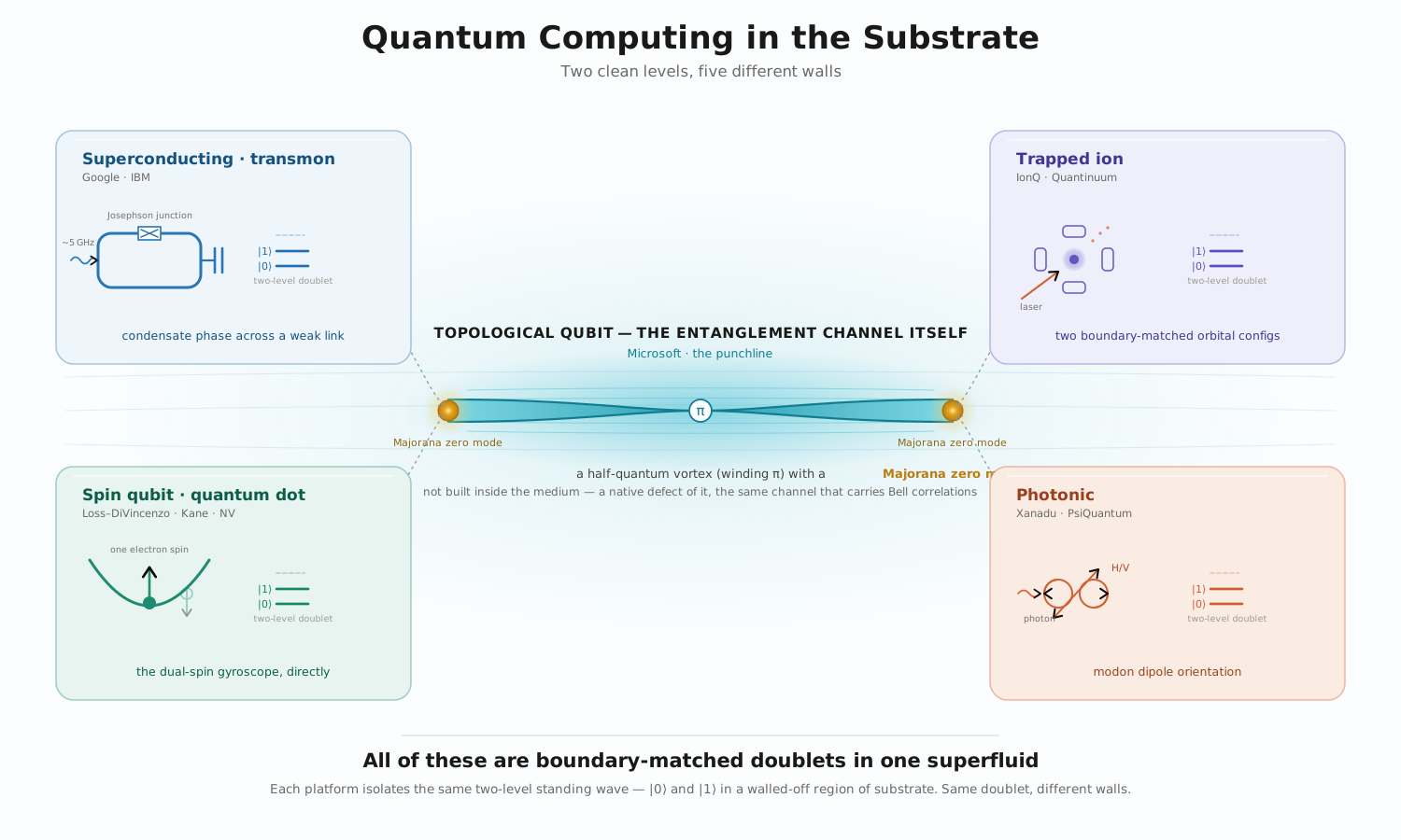
In the substrate, a qubit is the entanglement channel — the half-quantum vortex that carries Bell correlations between two separated particles — is a topological qubit. Same half-integer winding, same Majorana zero mode at the endpoints, same topological protection. The half-integer winding protects information in transit the same way it protects a qubit in a topological quantum computer.

Part 1: How a Qubit Is Actually Built

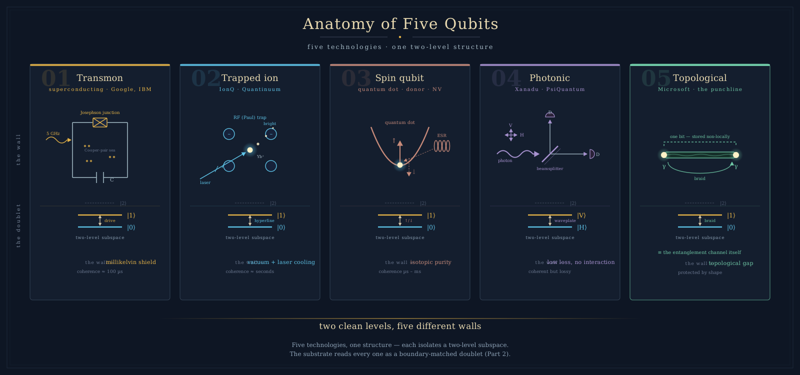
There is no single thing called “a qubit.” There are several physical systems, each with a two-level subspace that engineers isolate, control, and read. Knowing the hardware is the prerequisite for asking what the substrate says about it, so here are the five that matter, in the language of the labs that build them.

Superconducting (transmon) qubits — Google, IBM

The workhorse of the current era. Take a loop of superconductor interrupted by a Josephson junction — a thin insulating gap, a nanometer or two, that Cooper pairs tunnel across. A bare LC circuit is a harmonic oscillator: its energy levels are evenly spaced, so you can’t address just two of them. The Josephson junction makes the oscillator anharmonic — the rungs of the energy ladder become unevenly spaced — and you pick the lowest two rungs, |0\rangle and |1\rangle, separated by a microwave photon around 5 GHz. The “transmon” variant shunts the junction with a big capacitor to suppress charge noise.

You drive single-qubit rotations with shaped microwave pulses, you couple qubits through resonators or tunable couplers, and you read out the state by bouncing microwaves off a resonator whose frequency shifts depending on whether the qubit is in |0\rangle or |1\rangle. The whole chip lives at ~10 millikelvin in a dilution refrigerator, because the qubit splitting is tiny and any thermal photon scrambles it. Coherence times are tens to hundreds of microseconds.

The thing to hold onto: the computational degree of freedom is the phase of a superconducting condensate across a weak link. That will matter.

Trapped-ion qubits — IonQ, Quantinuum

Hold a single ion (ytterbium, calcium, barium) in a radio-frequency trap, in vacuum, and cool it with lasers until it is nearly motionless. The qubit is two long-lived internal electronic states of the ion — usually two hyperfine sublevels of the ground state, or a ground state and a metastable “clock” state. Lasers or microwaves drive rotations; you entangle two ions by using their shared motion in the trap as a bus (the Mølmer–Sørensen gate nudges the ions’ collective vibration in a state-dependent way). Readout is by fluorescence: shine a laser, and one qubit state scatters photons (bright) while the other stays dark.

Trapped ions have the longest coherence times in the business — seconds — and the cleanest gates, at the cost of speed and scaling difficulty.

The thing to hold onto: the computational degree of freedom is which boundary-matched orbital configuration the ion’s electrons sit in.

Spin qubits — quantum dots, donors, NV centers

The most literal qubit of all: a single electron’s spin, |\!\uparrow\rangle and |\!\downarrow\rangle. Trap one electron in a semiconductor quantum dot (Loss–DiVincenzo), or on a single phosphorus atom in silicon (Kane), or in the electron spin of a nitrogen-vacancy (NV) center in diamond. Manipulate it with oscillating magnetic fields (electron spin resonance) or, cleverly, with electric fields that move the electron through a magnetic gradient. Read it out by converting spin into charge or into a photon.

The thing to hold onto: this qubit is a single electron spin — which, in the framework, is exactly the dual-spin gyroscope. No translation needed; the substrate already has a complete mechanical model of this object.

Photonic qubits — Xanadu, PsiQuantum

Encode the qubit in a single photon: its polarization (horizontal/vertical), or which of two paths it took (dual-rail). Photons barely interact, which is wonderful for coherence and terrible for two-qubit gates — so photonic computing leans on measurement-induced interactions (the KLM scheme) or on continuous-variable “squeezed light.” Gates are beamsplitters, phase shifters, and detectors.

The thing to hold onto: the computational degree of freedom is the modon’s polarization — its dipole orientation. In the framework the photon is a modon, a counter-rotating vortex dipole, and its polarization is the orientation of that dipole.

Topological qubits — Microsoft, and the punchline of this chapter

The newest and most ambitious approach, and the one the entanglement sentence pointed at. Instead of storing the bit in any local property of one object, you store it non-locally, split between two Majorana zero modes — special zero-energy excitations that live at the ends of a topological-superconductor wire (or in the cores of certain vortices). One qubit is encoded in a pair of these modes. Because the information is in a global, topological property — not in any single place a stray field can reach — local noise cannot read it or corrupt it. You perform gates by braiding: physically moving the modes around each other, which transforms the stored state by an amount that depends only on the topology of the path, not its details.

This is the holy grail of fault tolerance: a qubit that is protected by the shape of its encoding rather than by heroic error correction. It is also the hardest to build, and as of the mid-2020s its experimental status is still being established and debated.

The thing to hold onto — and the rest of the chapter turns on it: a topological qubit is a pair of Majorana zero modes on a half-integer-winding defect. The substrate framework’s entanglement channel is a pair of Majorana zero modes on a half-quantum vortex. These are the same object.

Platform	Physical qubit	Coherence	What it is in the substrate
Transmon	Condensate phase across a Josephson junction	~100 μs	Boundary-matched doublet of a paired-condensate breathing mode
Trapped ion	Two internal electronic states	seconds	Two boundary-matched orbital-system configurations
Spin qubit	One electron spin	μs–ms	The dual-spin gyroscope, directly
Photonic	Photon polarization	long (lossy)	Modon dipole orientation
Topological	Pair of Majorana zero modes	(protected)	A half-quantum vortex channel — the entanglement channel itself

Figure 1: Five technologies, one structure. Each platform isolates a clean two-level subspace — the doublet — and walls it off from the rest of the world by a different means: a millikelvin shield, a vacuum trap, isotopic purity, low-loss optics, a topological gap. The apparatus differs; the structure does not. The substrate reads every one as a boundary-matched doublet (Part 2) — and the topological qubit (panel 5) as the entanglement channel itself.

Part 2: What a Qubit Is in the Substrate

Across five wildly different technologies, one structure repeats. The substrate explains why.

Every qubit is a boundary-matched doublet

Figure 2: One qubit, two standing waves. |0\rangle and |1\rangle are the two lowest boundary-matched modes of a little resonator in the substrate: an oscillatory interior joined smoothly — value and slope continuous — onto a decaying exterior at the wall. The matching admits exactly two clean low-lying solutions (|0\rangle with no interior node, |1\rangle with one); the would-be third is engineered far up in energy (anharmonicity), leaving a deliberately isolated doublet. It is the same boundary-matching that quantizes hydrogen orbitals and gives spin its two outcomes (l=\tfrac12 \to m=\pm\tfrac12).

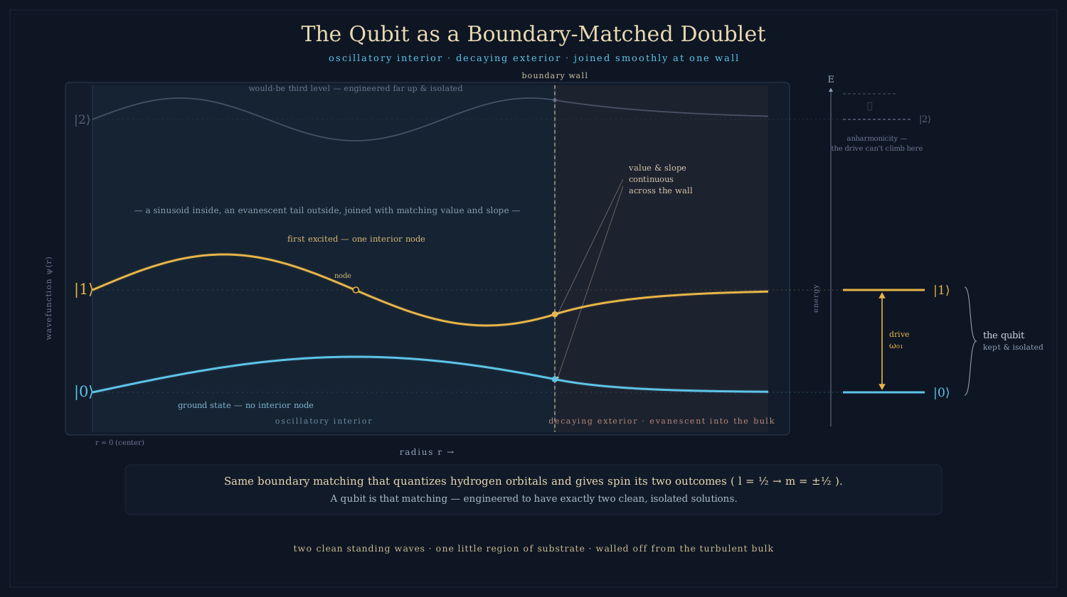
The framework’s signature move appears in chapter after chapter: a quantized state is a standing wave trapped between an oscillatory interior and a decaying exterior, joined at a boundary. Hydrogen orbitals come from this matching. The two outcomes of a spin measurement come from it — the l=1/2 matching at the electron’s single counter-rotating layer “has exactly two solutions,” m=\pm\tfrac12, and no intermediate values (Spin-Statistics). Modon energies come from it. It is the universal boundary-matching of the substrate.

A qubit is what you get when you engineer that matching to have exactly two clean, well-separated solutions and then isolate them from everything else. That is the entire art of qubit hardware: build a little resonator in the substrate whose boundary conditions admit a low doublet, push the third level far away (anharmonicity, in transmon language), and wall the doublet off from the turbulent bulk (millikelvin shielding, vacuum, isotopic purification — all the same job, done differently).

So the substrate’s first statement about quantum computing is unifying and almost mundane: a qubit is a deliberately clean two-state boundary-matched mode of the dc1 superfluid. |0\rangle and |1\rangle are two standing-wave configurations of the same little region of substrate. The transmon does it with a condensate phase across a weak link; the spin qubit does it with the dual-spin gyroscope’s two locked states; the ion does it with two electron-orbital configurations. Same doublet, different walls.

The transmon, read carefully, is already substrate physics

Figure 3: A transmon is the framework’s own pairing physics. Top — the device: a Josephson junction is two superconductors split by a thin insulator, Cooper pairs tunnelling the gap and the condensate phase \varphi winding across the weak link; shunted by a capacitor it becomes an anharmonic oscillator whose crowded rungs let a 5 GHz drive address only |0\rangle\leftrightarrow|1\rangle. Bottom — the substrate reading: the same two superconductors are seas of anti-phase breathing Cooper pairs — each pair two same-chirality electrons, one contracted (r_\text{eff}\approx150 fm) while its partner is expanded (\xi), so their net flow \approx 0 and the pair is a neutral, even-parity boson. The junction is a weak link where the paired-condensate order parameter may slip by 2\pi, and the qubit’s |0\rangle,|1\rangle are two boundary-matched states of that winding. The bridge is an identity: phase across the junction = winding of the paired-condensate order parameter.

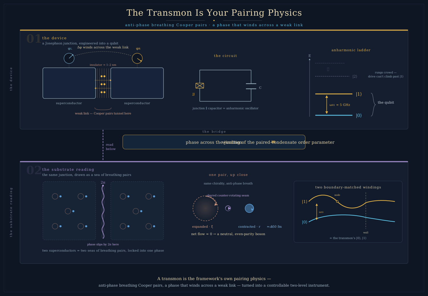
The transmon deserves a second look because it is built directly from objects the framework has already modeled. Its Cooper pairs are, in the framework, anti-phase Compton-breathing pairs — two electrons of the same circulation chirality breathing in opposite phase, one contracted while the other expands, so their combined flow averages to zero and the pair moves as a neutral, even-parity boson (Conductors; Spin-Statistics). The condensate is a sea of these breathing pairs locked into one macroscopic phase.

A Josephson junction is a place where that phase is allowed to wind — a weak link across which the superfluid order parameter can slip by 2\pi. The transmon qubit’s two levels are two boundary-matched states of this winding degree of freedom: the same physics as a vortex’s quantized circulation, miniaturized onto a chip and made anharmonic so you can address just the bottom two rungs. When a transmon “is in a superposition of |0\rangle and |1\rangle,” the framework reads that as a real, coherent breathing oscillation of the paired condensate — a macroscopic, engineered relative of the modon. A transmon is, quite literally, the substrate’s own pairing physics turned into a controllable instrument.

Spin qubits need no translation at all

Figure 4: The point on the Bloch sphere is the real orientation of a real gyroscope. Left — the abstract picture: the textbook qubit, a point |\psi\rangle = \alpha|0\rangle+\beta|1\rangle riding the surface of the Bloch sphere (|0\rangle north, |1\rangle south), with a single-qubit gate drawn as a rotation that sweeps the point along a latitude circle. Right — the substrate mechanism: the same object as the [dual-spin gyroscope](spin-stats.qmd) — an amber co-rotating core (Body 1) inside a teal counter-rotating boundary shell (Body 2), the net spin \mathbf{S}=\hbar/2 being the tiny residual L_\text{core}-L_\text{boundary}. The Bloch-vector rotation is the physical Larmor precession of \mathbf{S} about the applied field B (\omega_L=\gamma B — this is the gate), and the transverse nutation \Delta_+ — the core-against-boundary wobble — is [zitterbewegung](electron.qmd). Below — measurement: the boundary phase-locks to one of exactly two l=\tfrac12 solutions (m=\pm\tfrac12), the outcome fixed by the precession phase \varphi_0 at field onset — deterministic but unknowable below \tau_\text{lock}\sim10^{-21} s (contextual determinism). The qubit is never in two states at once.

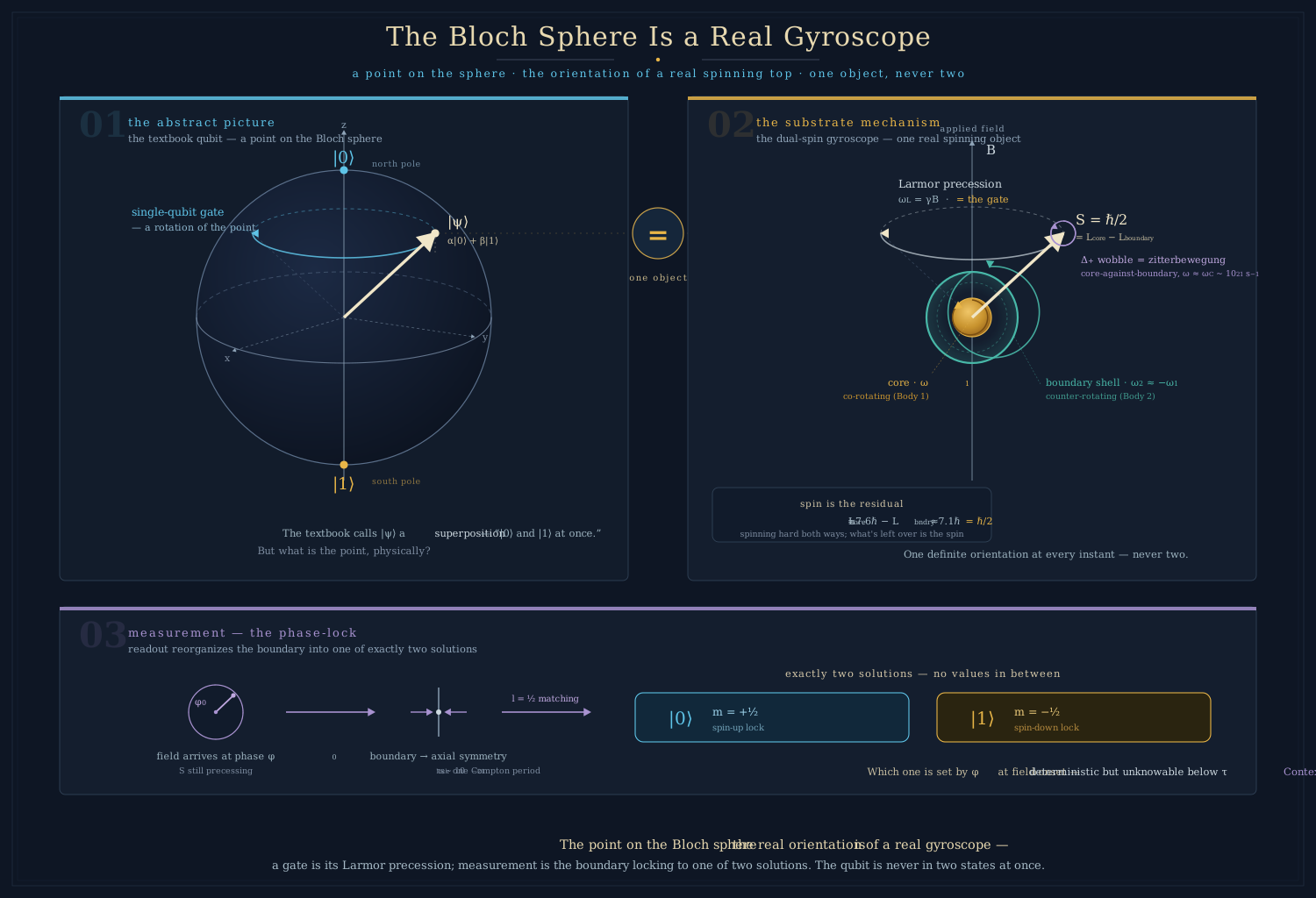
For a single-electron spin qubit, the framework’s model is already complete and quantitative. The two states are the dual-spin gyroscope’s two locked configurations. A single-qubit rotation is the net spin \mathbf{S} precessing around an applied field at the Larmor frequency, with the transverse nutation \Delta_+ being the internal core-against-boundary wobble — the same wobble the framework identifies with zitterbewegung. Measurement is the phase-lock: the boundary reorganizes into an axially symmetric pattern, and the outcome is set by the precession phase \varphi_0 at the instant the readout field arrives — “deterministic but practically unknowable,” what the spin chapter calls contextual determinism.

That last point is the hinge of Part 3, so it is worth stating sharply. In the substrate, the spin qubit is never in two states at once. It has, at every instant, one definite internal configuration. What looks like superposition is the real coherent precession of a real gyroscope, plus our ignorance of \varphi_0. Hold that thought.

Part 3: Superposition, and “All the Computations at Once”

Here is the question that motivated this chapter. The popular story says an n-qubit quantum computer holds 2^n numbers at once and evaluates them all in parallel — that a 300-qubit machine explores more states than there are atoms in the universe, simultaneously. Is that what is physically happening?

The substrate’s answer is no, not in that literal sense — and the reason is the same pilot-wave ontology that runs through the whole framework.

One history, one guiding field

Figure 5: Two ingredients, one scale up — and never “all the computations at once.” Top — one particle: the object (a modon, gold) is a beable that takes one definite path through one slit; its \xi-scale guiding field (the real ripple in \rho and S, cyan) spreads through both slits, interferes, and steers the object to a single bright fringe — one hit. Bottom — n qubits: the same two ingredients, scaled up. The hardware is n little objects, each in one definite configuration; above them sits a single real wave — the guiding field — carrying 2^n-component internal structure. Gates (violet) physically sculpt that one field; measurement reads one configuration out. There is no multiplicity of objects “trying every answer” — one history, plus a real field with exponential internal structure that gets shaped, then read.

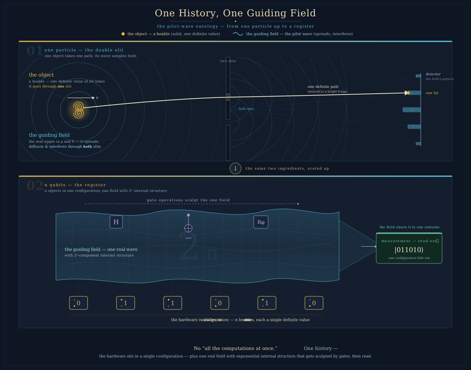
The framework is a pilot-wave theory of the de Broglie–Bohm family, given a physical medium. The wavefunction is not an abstract amplitude; it is \psi = \sqrt{\rho}\,e^{iS/\hbar}, with \rho the real density of the substrate and S the real phase of its flow. There are always two things, and they are different in kind:

• The objects — the actual modons, spins, condensate configurations. These are beables: they have definite values at all times. The electron goes through one slit. The spin sits at one orientation. The n physical qubits are, at every instant, in one definite joint configuration.
• The guiding field — the pilot wave, the \xi-scale perturbation envelope, the real ripple in \rho and S that surrounds the objects and steers them. This is what spreads, diffracts, and interferes.

In the double-slit chapter this resolves the oldest puzzle in the subject without paradox: the modon takes one path; its pilot wave samples both, interferes on the far side, and guides the modon to a bright fringe. There is no “particle in two places.” There is one particle and one wave, and the wave is doing the exploring.

A quantum computer is the same story, scaled up. The “superposition over 2^n basis states” is a structure in the guiding field, not a multiplicity of the objects. At every instant the machine’s physical hardware is in one configuration. The exponentially large object is the pilot wave’s interference pattern across the system’s configuration space — and a quantum algorithm is a recipe for physically sculpting that pattern (with gates) so that, when you finally let it steer the single physical configuration into a detector (measurement), the answer falls out with high probability.

So there is no literal “all computations at once.” There is one history. What there is, instead, is a real physical field with exponentially much internal structure, being shaped and then read.

Where to be careful — the field is real, and it does real work

The pilot wave is physical and its interference is real. In a pilot-wave account, the speedup of Shor’s algorithm is carried by the genuine, exponentially structured guiding field, which really does interfere in a way that concentrates amplitude on the factors. The framework predicts the same outputs as quantum mechanics, because it is quantum mechanics with a medium underneath (Bell’s Theorem makes this explicit: it reproduces -\cos\theta and S=2\sqrt2 exactly). Anything a real quantum computer can compute, the substrate predicts it can compute.

The substrate model separates two things the hype runs together: the resource, which is real and exponentially structured, and the story, which says a multiplicity of machines each try one answer. It keeps the first and drops the second. There is no parallel universe running the other computations — there is one real field with exponential internal structure, and one object steered by it.

Grover’s search, watched

The cleanest place to watch that distinction is Grover’s algorithm, because it is small enough to draw in full.

Grover’s is the needle-in-a-haystack problem. You have N items and a black box — an oracle — that answers yes or no about one item at a time. Nothing is sorted, so classically there is no better plan than trying items until one comes back yes: N/2 tries on average. Grover’s algorithm finds the needle in about \tfrac{\pi}{4}\sqrt N tries — for a phone book of a million entries, roughly 800 lookups instead of 500,000.

Take the smallest case worth drawing, and the one the simulation runs live: three qubits, so N = 8 possible readings, 000 through 111, one of them marked. Eight bars start equal, each at 1/8. Each turn of the algorithm makes exactly two moves:

1. The oracle flips the sign of the marked bar. The heights do not change at all — every reading is still 12.5% likely — so after this move alone there is nothing to read. What changed is invisible in the heights: the phase.
2. The diffusion reflects every bar about the average of all eight. The marked bar, now sitting below the average because its sign was flipped, comes back up above it; the seven unmarked bars, a whisker above the average, drop a whisker below.

Do that twice and 94.5% of the field is piled onto the marked item. Read the register out and it hands you the needle better than nine times in ten. Two things about that run are worth stopping on.

The hardware never splits. Watch the three arrows while the bars pile up. Each qubit has one orientation at every instant. The arrows shorten when the qubits entangle — their orientation has moved out of the qubits and into the channels between them — but at no point are there eight copies of anything, and at no point is a qubit in two places. The eight numbers being sculpted live in the guiding field, which is carried by the web of channels. Nothing in the scene is trying seven other answers.

And you can overshoot. Ask the simulation for a third turn and the answer gets worse:

Turns	1	2	3	4	5
P(marked)	78.1%	94.5%	33.0%	1.2%	54.8%

This is where the two stories part, and it is not subtle. If the machine were checking all eight answers at once, checking again could not make it worse — more parallel work is never negative. But if the algorithm is rotating one real wave by a fixed angle each turn, then of course it swings past the target and back: each turn rotates by \beta = \arcsin(1/\sqrt8) \approx 20.7^\circ, the chance of reading the marked item after k turns is \sin^2\!\big((2k+1)\beta\big), and k = 2 puts it at \sin^2(103.5^\circ) = 94.5\% — just past the peak at 90^\circ. Grover’s algorithm has to be stopped at the right moment, like a swing, and every engineer who implements it knows this. It is a rotation, and rotations come back around.

None of this contradicts standard quantum mechanics; the numbers are the textbook numbers, and the framework insists they must be. What it removes is the need to say the machine “tried all eight.” One object, one history, one real wave being turned — and a stopping rule, because the wave does not know when to stop.

The configuration-space problem becomes a channel-counting problem

Pilot-wave theories have a famous awkwardness: the guiding field lives in 3N-dimensional configuration space, not in ordinary 3D space. Where does a 3D superfluid keep a 2^n-dimensional object?

Figure 6: Where the 2^n lives. A pilot-wave theory has to keep a 2^n-dimensional guiding field somewhere — and a 3D superfluid has no room for it in the bulk. The substrate’s answer: it lives in the network of entanglement channels. Left, a product state — n qubits sitting apart, no channels, no high-dimensional structure; the field factorizes (\sim\!2n numbers). Middle, a partially entangled register — a few real [half-quantum vortex channels](bells-theorem.qmd) (winding \pi) woven between subsets. Right, a highly entangled register — a dense web of glowing laminar channels threading the substrate, now carrying the full 2^n-component amplitude. The correlations encode the high-dimensional object the way a hologram encodes a 3D scene on a 2D plate. Scalability is thereby reframed from a mathematical promise into a fluid-mechanical question: how many topologically protected channels can the medium sustain, coherently, against bulk turbulence?

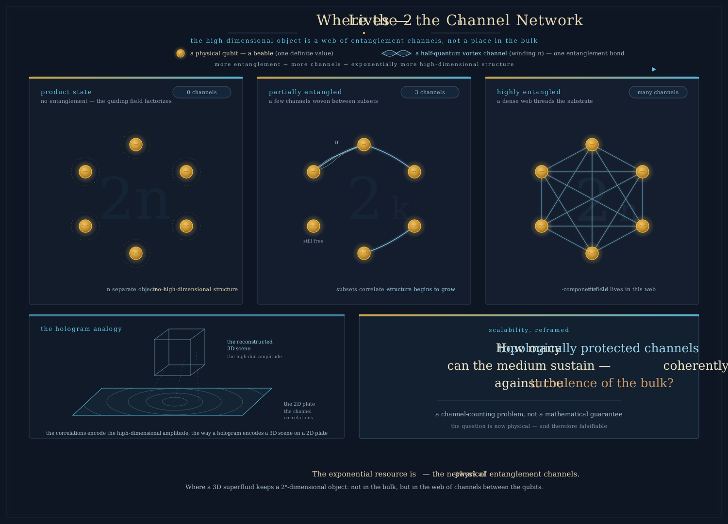
The substrate’s answer is the most interesting thing it has to say about quantum computing. The high-dimensional structure is not stored in the bulk fluid — it is stored in the network of entanglement channels between the physical qubits. Each two-qubit correlation the framework represents as a real half-quantum vortex channel threading the substrate between the parties. A product state has no channels; a maximally entangled register is a dense web of them. The “2^n-dimensional guiding field” is physically the pattern of these vortex channels and their phases — a real, finite, 3D-embedded structure that encodes the high-dimensional amplitude through its correlations, the way a hologram encodes a 3D scene on a 2D plate.

This reframes scalability from a mathematical promise into a fluid-mechanical question:

How many topologically protected vortex channels can the substrate sustain, coherently, against the turbulence of the bulk?

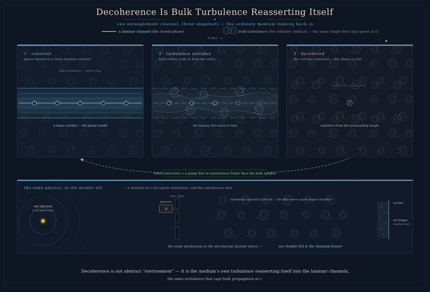
Decoherence, in this picture, is not abstract “interaction with the environment.” It is the bulk substrate reasserting itself — the tangled counter-rotating structure of the ordinary medium leaking back into the laminar channels and unwinding them, the same turbulence that limits bulk propagation to c and that a detector at a slit injects to kill interference. Every error-correction scheme is, in substrate language, a pump that re-laminarizes channels faster than turbulence tangles them.

Figure 7: Decoherence is the bulk reasserting itself. A single entanglement channel, read across three snapshots. Stage 1 — coherent: a clean glowing laminar corridor holds the stored phase (the aligned clocks on its centerline), while the bulk’s tangled counter-rotating eddies are swept clear of the walls and held at bay. Stage 2 — turbulence intrudes: tendrils of the bulk eddy structure leak in from the walls, the laminar streamlines begin to fray, and the phase clocks slip out of alignment. Stage 3 — decohered: the corridor is unwound, indistinct from the surrounding tangle, the stored phase lost. The green feedback loop names error correction physically — a pump that re-laminarizes the channel faster than the bulk can re-tangle it. Below, the same mechanism in miniature: a [detector at a slit](double-slit-quantum-eraser.qmd) injects turbulence that kills the interference, exactly as it kills the channel above.

Part 4: Entanglement, Two-Qubit Gates, and the Piano Wire

Single qubits are easy; the power is in entanglement, and entanglement is where the framework is most concrete. From the Bell chapter: when two systems are entangled, they are joined by a real half-quantum vortex in the substrate’s SU(2)\to U(1) order parameter — a filament whose order parameter winds by \pi, not 2\pi, around its axis. The half-integer winding is the singlet constraint, recorded in the substrate’s geometry, and it is topologically protected: no local, continuous deformation can unwind it.

A two-qubit entangling gate (a CNOT, a Mølmer–Sørensen, a controlled-phase) is, physically, the operation that carves, links, or twists these channels between two qubits’ orbital systems. Creating entanglement carves a channel. A controlled-phase imprints a relative phase along it. Disentangling annihilates it. The entire circuit model — the dance of CNOTs that builds up a computation — is, in the substrate, a choreography of vortex channels being woven and rewoven through the medium.

The channel interior is a laminar corridor, swept clear of the counter-rotating obstacles that clog the bulk — so disturbances on it are not limited to c. They are twist waves — torsional zero modes bound to the core of a half-quantum vortex line, not ordinary Kelvin bending waves, which are capped below c — and their speed is bounded by direct experiment at v_\text{ch} > 5\times10^6\,c, plausibly of order the mass ratio m_e/m_1 \approx 2.5\times10^8 (Bell, Part 2). The wire is strung taut by topological tension; when measurement “cuts” one end, the twist snaps down the line faster than c and resets the far end — the piano wire that, when cut, snaps back faster than light. The 10^9-fold scaleup you already invoke for the electron’s wake is the same hierarchy: a microscopic medium carrying structure for a macroscopic object, with the channel inheriting the substrate’s microscopic velocity scale rather than its collective one.

Two consequences for computing follow directly:

• No-cloning has a mechanical reason. You cannot copy an unknown qubit because the information is held in the winding and phase of a topological channel, and a channel cannot be locally duplicated — copying it would require a 2\pi structure to decompose into two \pi structures, which the topology forbids. This is the same selection rule that protects the twist wave in transit.
• The entangled resource is fragile in a specific, predicted way. Channels have finite coherence length and finite signalling speed v_\text{ch}, with a maximum useful range L_\text{max} = v_\text{ch}\,\Delta t — \Delta t the window within which the two endpoints are acted on simultaneously in the substrate frame — beyond which the channel cannot keep its endpoints synchronized before they are measured. The Bell chapter already turns this into a falsifiable prediction (correlations degrading past L_\text{max}). For a computer, the same finiteness becomes a fundamental error floor.

Part 5: The Topological Qubit Is the Entanglement Channel

Recall the topological qubit: a bit stored non-locally in a pair of Majorana zero modes on a half-integer-winding defect, protected because the information lives in the defect’s global topology.

Recall the framework’s entanglement channel: a half-quantum vortex whose half-integer winding carries a Majorana zero mode at each endpoint (the framework’s fermions are Alice strings on a ^3He-A-class order parameter, each carrying a Majorana zero mode — Substrate Particles, with the Ivanov/Read–Green grounding in Open Problems). The twist wave that propagates A’s measurement to B is a zero mode bound to the vortex core, protected by an Atiyah–Singer index theorem (Bell, Part 3) — “the same mathematics that protects qubits in topological quantum computers.”

These are not two things that resemble each other. They are the same physical object, used two ways:

	Substrate entanglement channel	Topological qubit
Defect	Half-quantum vortex (winding \pi)	Topological-SC wire / vortex (winding \pi)
Stored at	Two endpoints	Two Majorana zero modes
Protection	Half-integer modes can’t decompose into integer bulk modes	Topological gap; non-local encoding
Operation	Measurement launches a protected twist wave	Braiding transforms the encoded state
What forbids errors	Topological selection rule	Topological selection rule

When Nature wants to correlate two distant particles, it grows one of these channels and lets it sit. When an engineer wants to store and compute on a qubit with maximal protection, they grow one of these channels and braid its endpoints. The topological quantum computer is the substrate’s own entanglement mechanism, harnessed deliberately. This is why, of all the platforms, the topological qubit is the one the framework regards as most fundamental: the transmon and the spin qubit are clean doublets the engineer builds inside the substrate; the topological qubit is the engineer reaching down and manipulating a native defect of the substrate itself — the very structure the framework already uses to explain Bell correlations.

It also means the framework makes a quiet, strong claim about the field’s roadmap: braiding works because half-quantum vortices and their Majorana modes are real substrate objects with real topological protection — the framework needs them to exist anyway, to explain entanglement and the half-integer winding of fermions. If topological qubits are eventually built and braided cleanly, the framework reads that not as a surprise but as a direct manipulation of the medium it has been describing all along.

Part 6: Where Quantum Computing Works, and Where the Substrate Predicts a Wall

The framework is a refinement of quantum mechanics, not a rival: it reproduces every measured quantum result and departs only at extreme regimes (Bell’s Theorem). So the substrate cannot, and does not, say “quantum computers can’t work.” Within its coherence limits it predicts they work exactly as quantum mechanics says. What it adds is a physical account of where those limits are — and three sharp, separable statements.

1. Quantum random number generation is rock solid — and now has a physical source

A quantum random number generator harvests the randomness of measurement outcomes. In the substrate, that randomness is not a mathematical axiom; it is real entropy drawn from substrate microstructure — the precession phase \varphi_0 at the instant of the phase-lock, set by the qubit’s history and the local substrate flow, deterministic but genuinely unknowable below the Compton-scale locking time \tau_\text{lock}\sim10^{-21} s (Spin-Statistics). A substrate QRNG is sampling the chaotic, frame-dependent state of the medium at a timescale no apparatus can resolve. This is the cleanest possible entropy source — better-founded than thermal noise, because it bottoms out at the substrate’s own dynamics. Your instinct that quantum randomness for cryptography “is still solid” is, in this framework, more than solid: the substrate explains why it is trustworthy.

2. “Quantum supremacy” by sampling is real but is mostly an entropy demonstration

The headline “supremacy” demonstrations (random-circuit sampling) prove that a quantum device can sample from a probability distribution too complex to simulate classically. In the substrate, that is exactly what it is: the machine is a physical instrument for sampling a fiendishly structured interference pattern in the guiding field. It is genuine, it is hard to fake — and it is not, by itself, a useful computation. It demonstrates that the medium can hold and sample exponential structure. Whether that structure can be steered to a useful answer (factoring, simulation) rather than merely sampled is the separate question of algorithmic, fault-tolerant computing — and a much harder bar.

3. The distinctive, falsifiable claim: a fundamental coherence floor

Idealized quantum mechanics promises that with enough error-correcting overhead, a coherent computation can be made arbitrarily large — the fault-tolerance threshold theorem assumes errors are independent and bounded, and below threshold the logical error rate can be pushed as low as you like. The substrate questions the premise. Because entanglement is carried by physical vortex channels with finite coherence and a finite range L_\text{max} = v_\text{ch}\tau, and because decoherence is the bulk turbulence reasserting itself into those channels, the framework predicts a physical floor on how much coherent entanglement the medium can sustain at once — a floor that is not of the independent-error form the threshold theorem assumes, because the bulk is a shared medium and its reassertion can correlate errors across channels.

In sharp form:

Substrate prediction. There exists a scale of coherent entanglement — a combination of qubit count, circuit depth, and physical extent — beyond which error rates stop falling with better engineering and saturate at a substrate-set floor, because the bulk medium tangles channels faster than any code can re-laminarize them. Idealized QM predicts no such floor.

With the substrate framework, scalable fault-tolerant factoring (Shor at cryptographic size) runs into a physical wall that pure quantum mechanics says isn’t there — and the location of that wall is a property of the substrate, in principle measurable.

This is currently consistent with all data, because today’s machines are nowhere near the fault-tolerance threshold; their errors are dominated by ordinary engineering noise, which masks any fundamental floor. The two pictures — “engineering noise, beatable” versus “substrate floor, fundamental” — only separate as devices improve. The framework’s bet is that as error rates are pushed down, they will stop at a floor with a fluid-dynamical signature: errors that correlate across the chip in a way that tracks substrate structure (the \xi\approx100\,\mum coherence length, the d_\text{GJO}\approx16\,\mum sheet spacing, the L_\text{max} of the Bell prediction) rather than the spatially independent noise the threshold theorem assumes.

Where the floor bites depends on the pitch. The simulation’s third view makes the prediction concrete and, in doing so, sharpens it. Put a d\times d code on a chip at a platform’s real qubit spacing, let the bulk’s weather — eddies of the cell size \xi, and larger ones in the Kolmogorov range above it — drift over it, and let every qubit under an intruding eddy err together, at a per-qubit rate held fixed so that the only new ingredient is the correlation. A code corrects up to (d-1)/2 errors per round; a gust that covers more than half a row cannot be voted away, and the logical error stops falling at the rate of such gusts, however good the engineering. Whether a gust can do that is a ratio, gust size against qubit pitch, and the platforms sit on both sides of it. Trapped ions, neutral atoms, and spin qubits pack hundreds to thousands of qubits into one cell, so a single cell-sized intrusion takes a whole row and the floor sits at the substrate’s own rate whatever the code distance. Transmons at \sim1 mm pitch put ten cells between neighbours, so cell-sized intrusions land one qubit at a time and are corrected like any other noise — no floor — unless the cascade supplies eddies wider than the pitch, or the substrate wind lines up with a code row. That last case is the sharpest signature the framework offers. The substrate frame is the CMB frame (Michelson–Morley), so the lab moves through the weather at 370 km/s, a cell crosses a qubit in \xi/v\approx0.3 ns, and one code cycle sweeps tens of centimetres of substrate past the chip: an intrusion is a streak along the wind, not a spot, and it defeats a code only when the wind runs along the code’s rows. The apex of the CMB dipole is fixed on the sky, so on a chip fixed in the lab the wind direction turns with the sidereal day — and so should the correlated-error rate, a modulation with a 23 h 56 m period aligned to Leo that no engineering noise shares. The height of the floor is not derived here; its geometry is.

Summary

Question	Popular framing	Substrate framing
What is a qubit?	An abstract two-level system	A deliberately clean boundary-matched doublet of the superfluid
What is superposition?	Being in two states at once	One object in one configuration; a real pilot wave with two-component structure guiding it
“All computations at once”?	Exponential parallelism, many worlds	One history; one real guiding field with exponential internal structure, sculpted then read
Where does the 2^n structure live?	Abstract Hilbert space	The physical network of entanglement channels (half-quantum vortices)
What is entanglement?	Nonlocal correlation	A real half-quantum vortex channel in the substrate
What is a two-qubit gate?	A unitary on Hilbert space	Carving, linking, or twisting vortex channels
What is decoherence?	Interaction with environment	Bulk turbulence reasserting itself into laminar channels
What is a topological qubit?	Majorana modes on a defect	The entanglement channel itself, harnessed
Is quantum RNG trustworthy?	Yes, by postulate	Yes, and the substrate gives it a physical entropy source (contextual determinism)
Will QC scale arbitrarily?	Yes, above threshold	Predicts a physical coherence floor with a fluid-dynamical signature — falsifiable

The throughline: quantum computing is, in this framework, the engineering of a superfluid. Its qubits are clean doublets cut into the medium; its entanglement is real vortex channels; its protection mechanisms (topological qubits, error correction) are the medium’s own topology and a fight against the medium’s own turbulence. The framework demystifies the philosophy — there is one history, not a multiverse of parallel computations — without deflating the physics, since the real guiding field genuinely carries exponential structure. And it makes one prediction that idealized quantum mechanics does not: that the medium has a finite capacity for coherent entanglement, and that scaling will eventually find its floor.