Double-Slit Experiment & Quantum Eraser

The Double-Slit Experiment

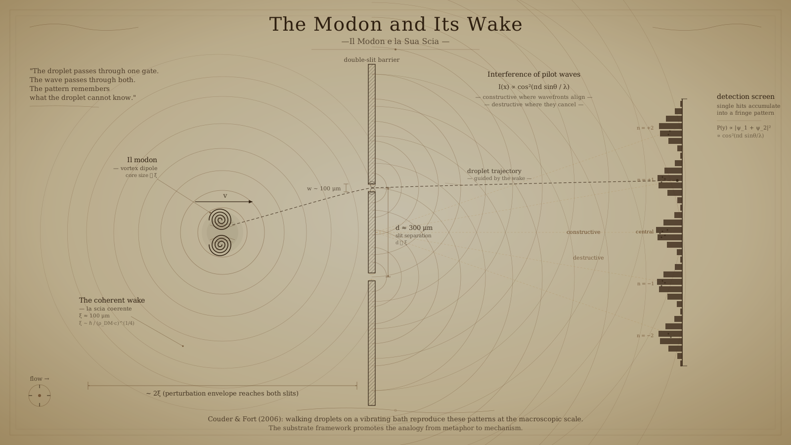
Pilot wave interference in the substrate’s perturbation envelope

Interactive: open the double-slit simulation — fire modons one at a time, watch the pilot wave go through both slits while the core goes through one, cut its coherent tail down to one cell and back up to a free wave to see what the measured fringes demand, put a detector on a slit and turn its coupling up, and step inside a lattice cell to see why the ripple is so easily disturbed.

The Standard Mystery

Fire single photons at a barrier with two narrow slits. Detect them one at a time on a screen behind the barrier. Each photon arrives as a single point — a discrete detection event. But accumulate enough detections and an interference pattern emerges: bright bands where photons cluster, dark bands where they never land.

Close one slit and the pattern disappears — you get a single broad hump. Open both slits and the fringes return. The photon apparently “knows” whether both slits are open, even though it arrives as a single localized click.

Now add a detector at one slit — anything that records which slit the photon passed through. The interference pattern vanishes. The photon still arrives one at a time, but the fringes are gone — replaced by two overlapping humps, as if each photon went through one slit or the other with no wave behavior at all.

Standard quantum mechanics describes this perfectly with the wavefunction formalism but offers no mechanism. The photon is neither a wave nor a particle; it is a probability amplitude that passes through both slits, interferes with itself, and collapses upon detection. The “measurement problem” — why does observing the slit destroy the interference? — has generated nearly a century of interpretive debate.

The Substrate Explanation

In the substrate framework, the photon is a modon — a compact counter-rotating vortex dipole whose energy is concentrated in two vortex cores far smaller than the coherence length (see The Photon as Modon). The modon is a localized object. It goes through one slit. There is no mystery about “which path” the energy takes.

But the modon does not travel alone. It displaces the dc1 substrate as it propagates, creating a perturbation envelope of radius \xi \approx 100\;\mu\text{m} — the “boat in the harbor” effect described in Emergent Speed of Light — and, trailing that envelope, a coherent tail: the ripple the envelope has already launched, which spreads like any wave and reaches far beyond \xi (below). Envelope and tail together are the pilot wave: a coherent ripple in the substrate’s density and phase field that surrounds the compact dipole core and mediates its interaction with the environment.

The envelope is enormous compared to the modon core, and comparable to the slit geometry of a real experiment (slit widths of order 0.1 mm, separations of 0.1–1 mm). What spans both slits at those separations — and at the metres of a stellar interferometer — is the tail. The pilot wave diffracts through both openings even though the modon core passes through only one, interferes on the far side, and creates a structured guidance field that steers the modon toward the bright fringes and away from the dark ones.

This is not speculation — it is exactly what happens in the walking-droplet experiments of Bush, Couder, and collaborators.¹ A millimeter-scale oil droplet bounces on a vibrating fluid surface, generating a pilot wave that extends far beyond the droplet itself. When the droplet-plus-wave encounters a double-slit barrier, the droplet passes through one slit but the wave diffracts through both, and the resulting interference pattern in the wave field guides the droplet’s trajectory. Over many runs, the droplet positions reproduce the quantum interference pattern.

The substrate framework promotes this from analogy to mechanism: the dc1 superfluid is the vibrating bath, the modon is the droplet, and the \xi-scale perturbation envelope with its coherent tail is the pilot wave. The interference pattern is a real, physical pattern in the substrate’s density field — not a probability amplitude, not an abstraction, but a fluid flow structure that pushes the modon toward constructive interference regions and away from destructive ones.

The Coherent Tail: How Far the Pilot Wave Reaches

The pilot wave has two parts, and the experiments measure the second one.

The envelope is the fresh displacement: the \xi-wide ripple the core is making right now, regenerated at every cell it crosses — the boat’s own bow wave. The cell view of the simulation shows what it costs: nothing. Each sheet is pushed out as the envelope passes and springs back behind it; a 2.5 eV photon is a millionth of the 1.7 MeV one cell already holds, and no energy changes hands.

The tail is what the envelope leaves behind. A displacement made in a superfluid does not stay where it was made. It propagates at c, and since the core also moves at c, the ripple launched at every point of the flight travels with the modon while spreading sideways. What leaks out of the envelope is not energy but phase: the modon’s winding threads the cells the envelope has swept, and the lattice’s own vortex lines carry that phase outward as coherent ripples — the same “winding stretched thin” that carries light below the floor, and the same long-range vortex-line coherence that the Outer Reach reads at \ell_L \approx 3.9 cm. Two things about the tail matter for the double slit.

• It is ordered, not turbulent. The tail is a phase pattern spread over an enormous number of cells with almost no energy in any of them. That is exactly what lets it interfere, and exactly what makes it the most fragile object in the framework: any boundary that intrudes re-phases it. The detector does not find turbulence in the tail; it makes turbulence out of it.
• It does not die. In the walking-droplet experiments the reach of the pilot wave is set by the bath’s memory — how many bounces a surface wave survives before viscosity erases it — and every quantum-like behaviour appears only at high memory (Silicone Oil Bath). The substrate’s memory is not a tuned parameter. The medium is lossless, and the same topological protection that lets a photon cross the universe at c without dispersing keeps its tail coherent for as long as the photon exists. The substrate is the bath’s infinite-memory limit.

What the experiments say about the reach. Single-photon interference has been observed across two openings whose separation, in units of the cell, runs from a handful to millions:

experiment	what is separated	separation	in cells \xi	source
Young double slit, heralded photons (Luo, Galvez et al. 2024)	two slits 0.13 mm wide, 3 m to the detector	0.62 mm	6.4	down-conversion pairs, 810 nm
weak-measurement trajectories (Kocsis et al. 2011)	two 0.6 mm beams, imaged 2.75–8.2 m downstream	4.69 mm	48	quantum dot, 943 nm
Michelson–Pease stellar interferometer (1920)	two mirrors on a beam	6.1 m	6\times10^4	Betelgeuse
CHARA array (2001)	two telescopes	331 m	3\times10^6	starlight

The double-slit row is a tabletop demonstration with heralded photon pairs;² the Kocsis row is the experiment whose weak-measurement trajectories are cited below, in which single photons from a quantum dot were split by a fibre beamsplitter into two collimated beams 4.69 mm apart and their average paths followed over more than five metres.³ The stellar rows are single-photon rows too: at optical frequencies starlight carries far fewer than one photon per mode (below 10^{-3} for a red supergiant like Betelgeuse), so each detected photon’s wave arrived at both telescopes essentially alone — and, per Dirac, interfered only with itself.⁴ Along the flight the same holds: Grangier, Roger and Aspect’s single photons from an atomic cascade interfered in a Mach–Zehnder with visibility above 98%,⁵ and Jacques et al. sent single photons from a nitrogen-vacancy centre down two spatially separated 48 m paths (160 ns of flight) and recovered V = 93 \pm 2\%, with V^2 + D^2 = 0.97 \pm 0.03 against the which-path distinguishability D.⁶

Three conclusions follow, and none of them is a fit.

1. No substrate length cuts the tail off. The tabletop double slit exceeds \xi; Kocsis exceeds the dc1 thermal de Broglie length \lambda_\text{dB} \approx 1.3 mm = 13\,\xi; the stellar baselines exceed the outer reach \ell_L \approx 3.9 cm = 400\,\xi by two to four orders of magnitude. Whatever \ell_L bounds for the substrate’s own sub-floor modes, it does not bound the pilot wave of a photon far above the floor. The simulation’s tail slider therefore defaults to a free, unbounded wave; its shorter settings exist to show what a cutoff would do to the fringes.
2. Far from the source, the tail is the wave. Two openings fed with amplitudes A and tA give fringes of visibility V = 2t/(1+t^2), so V = 0.93 needs t \ge 0.68 and V = 0.98 needs t \ge 0.82. Where the two paths are fed by a beamsplitter the amplitudes are equal by construction, and those are the visibilities measured — over 48 m of flight in Jacques’ case. Where two openings sit in free space, a double slit or a stellar baseline, the fringes are what wave optics gives for equal illumination of both openings; any extra amplitude the fresh envelope adds at the slit the core goes through must be small enough to leave that unspoiled. By the time the wave reaches a slit, the harbour is all wake.
3. The reach scales with the flight and with the colour the way a wave’s does. A tail launched from a region of size a spreads to a transverse width of order \lambda L/a after a flight L; for an extended source it is the van Cittert–Zernike coherence width. Redder photons reach farther across for a given flight, not less. Photon energy enters the tail as the depth of the displacement — how strongly the phase is written into each cell — not as how far it reaches.

What \xi still does. The envelope is a near-field object. A \xi-wide source of green light has a Rayleigh range \pi\xi^2/2\lambda \approx 3 cm (a number that scales as 1/\lambda and is not \ell_L); only inside it, with the slits within centimetres of the emitter, does the fresh envelope carry a share of the wave comparable to the tail. Beyond it the envelope is the local bow wave riding on a much wider wake, and \xi is what the core sees: the scale on which the lattice averages to a smooth medium (Emergent Speed of Light). What the envelope adds to the wave-optics amplitude at the slits inside that near field is the one place a substrate length could leave a fingerprint on a double-slit pattern, and it is an open computation (Quantitative Status).

NoteHonest accounting

The tail’s persistence is a framework claim (a lossless, topologically protected medium), and the numbers in the table are lower bounds on its reach read from existing data, not predictions. Everything in the reach column is what wave optics already assigns to the photon’s wavefunction; the substrate reproduces it by being a linear wave-bearing medium at these amplitudes, and adds nothing to it at these scales. The vortex-line picture of how phase leaves the envelope — the winding threading the swept cells, carried outward along the lattice’s own lines — is the framework’s mechanism, consistent with the Outer Reach but not derived here. And the chapter does not have a derivation of t, the tail’s amplitude relative to the envelope, as a function of flight and geometry: the simulation sets it from the measured visibilities (t_0 = 0.75, a coherent V \approx 0.95), and computing it from the substrate’s hydrodynamics is the diffraction calculation the Quantitative Status already owes.

Why Measurement Destroys Interference

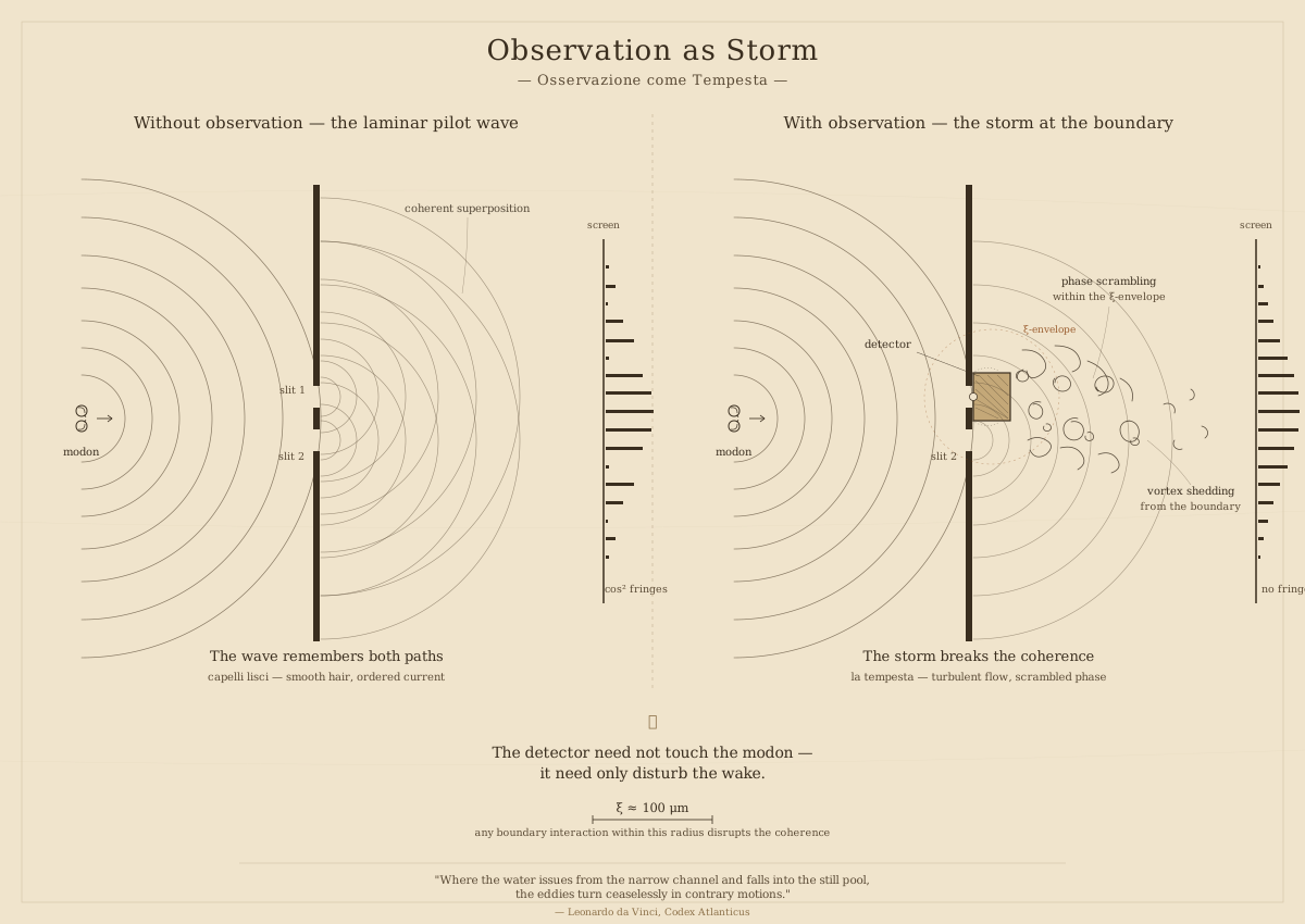
Place a detector at one slit. In the substrate framework, the detector is a macroscopic boundary — an arrangement of baryonic matter coupled to the substrate through its own orbital system complexes. When a photon’s perturbation envelope passes through the slit, the detector’s boundary layers interact with the substrate flow within the \xi-scale envelope.

This interaction is not gentle. The detector is a turbulent intrusion into the coherent pilot wave field. The substrate flow near the observed slit becomes disordered — the organized phase structure of the pilot wave is disrupted by the detector’s own boundary dynamics. In the language of superfluid hydrodynamics, the detector creates vortex shedding and phase scrambling within the perturbation envelope at the monitored slit.

The result: the pilot wave component passing through the observed slit loses its phase coherence. It can no longer interfere constructively or destructively with the component passing through the other slit. The fringes disappear — not because “the wavefunction collapsed,” but because the medium was locally disturbed. The modon still arrives at the screen as a point detection, but without a coherent pilot wave to guide it, its landing positions follow the classical pattern: two overlapping humps.

The coherence domain is the whole pilot wave, tail included — not the \xi envelope alone. That is why a detector at either slit kills the fringes: the slit the core did not pass through carries only tail, and re-phasing that tail is enough. The core itself is never touched. It carries its energy through its own slit whole, rides the far-side field exactly as before, and lands as a single click; what changed is that the field it rides no longer has a coherent partner from the other slit to interfere with. The measurement does not need to “touch” the modon core or absorb the photon — it only needs to introduce disorder into a phase pattern that carries almost no energy, at either slit, and the interference is gone. The \xi \approx 100\;\mu\text{m} scale is where that fragility comes from: a green photon’s ripple is a millionth of the energy a single cell holds, spread across every cell the tail threads, so any boundary that intrudes into it is overwhelmingly stronger than the thing it disturbs.

This also explains the gradual degradation observed in weak measurement experiments:⁷ a weak coupling to the pilot wave introduces less turbulence than a strong one. The interference fringes degrade smoothly as the measurement strength increases, exactly as expected if the mechanism is progressive disruption of a fluid coherence structure rather than a discrete “collapse.”

The Quantum Eraser

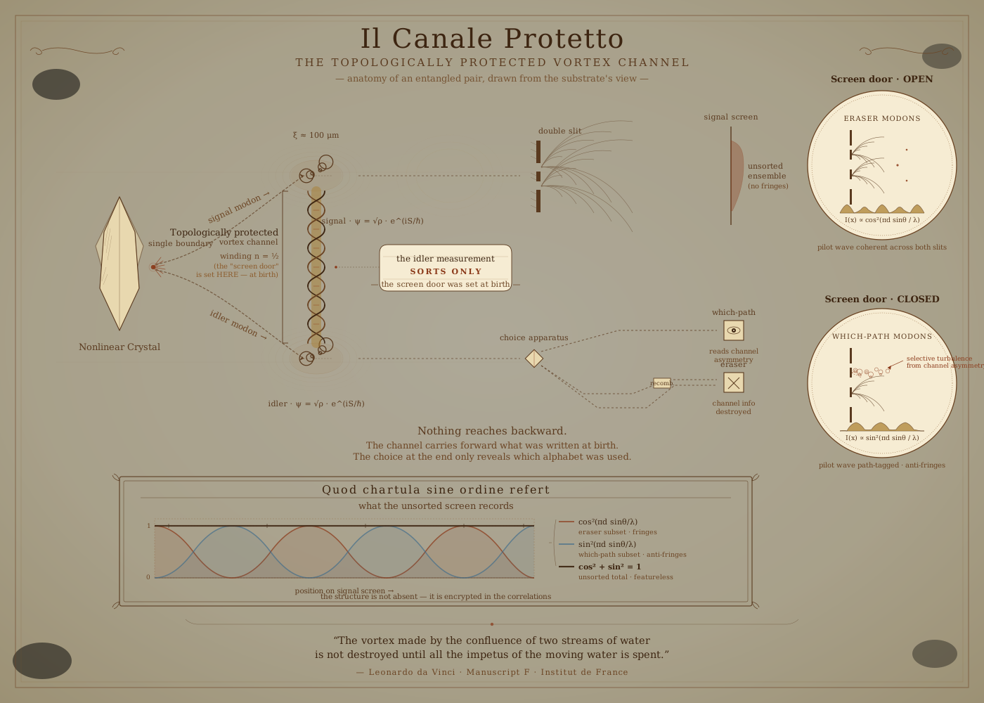
Correlated channel topology in the substrate

The Standard Mystery

The delayed-choice quantum eraser⁸ takes the double-slit mystery a step further. Generate an entangled photon pair. Send the signal photon through the double slit to a detector screen. Send the idler photon to a separate apparatus that can either measure which-path information or “erase” it by combining the two path-tagged beams before detection.

The results:

• The total pattern of signal photon detections — all of them, unsorted — is always a featureless blob. No fringes.
• Sort the signal detections by what happened to their idler partners. For idlers whose which-path information was erased, the corresponding signal photons show an interference pattern. For idlers whose which-path information was preserved, the corresponding signal photons show no fringes — just the two-hump classical pattern.
• The idler measurement can happen after the signal photon has already been detected. The choice to erase or preserve seemingly reaches backward in time to affect the signal photon’s behavior.

This apparent retrocausality has generated enormous philosophical debate. Standard quantum mechanics handles it cleanly through entanglement correlations — no signal is actually sent backward — but the physical mechanism remains opaque.

The Substrate Explanation

The substrate framework explains the quantum eraser without retrocausality, using two elements already established in the model: the pilot wave (from the double-slit explanation above) and the topologically protected vortex channel that connects entangled particles (from the entanglement mechanism).

Step 1: Entangled pair creation. When the entangled pair is generated (typically by spontaneous parametric down-conversion in a nonlinear crystal), the two photon-modons are created from a single boundary reorganization event. They emerge connected by a topologically protected vortex channel in the substrate — a filament of organized substrate flow whose half-integer winding number protects it from decoherence. This channel is the substrate’s physical realization of entanglement.

Crucially, the channel’s topology is established at creation. The two modons share correlated internal states from the moment they separate — their vortex orientations, phase relationships, and boundary structures are locked together by the channel’s winding number. This is not a hidden variable in the classical sense (it is a nonlocal substrate structure), but it is a physical structure with definite properties at all times.

Step 2: The signal photon at the double slit. The signal modon encounters the double slit. Its \xi-scale perturbation envelope diffracts through both slits, as before. But now the pilot wave carries additional structure: the phase signature of the entanglement channel. This channel topology effectively tags each component of the pilot wave with information about the pair’s shared state.

The total ensemble of signal photons contains two sub-populations, distinguished by their channel topology:

• Photons whose idler will encounter the eraser path have a channel topology that preserves pilot wave coherence across both slits. Their pilot waves interfere normally.
• Photons whose idler will encounter the which-path detector have a channel topology that is correlated with which slit the modon’s pilot wave is most strongly coupled to — a selective turbulence pattern, like a screen door over the slit geometry, where the channel state determines which spatial modes carry coherent phase and which carry disorder.

Both sub-populations hit the signal screen. Their fringes and anti-fringes sum to a featureless blob — the total pattern. The interference information is present in the substrate’s flow structure, but it is encrypted in the channel correlations and invisible in the unsorted data.

Step 3: The idler measurement sorts the ensemble. When the idler photon is measured — either in the which-path basis or the eraser basis — the measurement outcome serves as a sorting key. It does not send a signal backward to the signal photon. It identifies which sub-population each signal detection belongs to.

In the eraser configuration, the idler’s which-path information is destroyed by recombining the two possible paths before detection. Only idlers whose channel topology was compatible with coherent pilot wave interference at the signal slit pass through this configuration symmetrically. Sorting by these idler outcomes selects the sub-population whose signal photons had coherent pilot waves — and the fringes appear.

In the which-path configuration, the idler reveals which slit the signal photon’s pilot wave was predominantly coupled to. Sorting by these idler outcomes selects the sub-population whose signal photons had path-tagged pilot waves — and no fringes appear.

Step 4: No retrocausality. The key insight is that the channel topology is established at pair creation, before either photon reaches its detector. The signal photon’s pilot wave structure at the double slit is determined by the channel state at the moment of emission — not by a future measurement on the idler. The idler measurement does not change anything about the signal photon’s history. It reveals which sub-ensemble the signal photon belonged to all along.

This is the substrate’s resolution of the apparent backward-in-time effect: the correlated channel topology creates sub-populations with different pilot wave coherence properties at the slit. The idler measurement sorts these sub-populations. The fringes were always there in the sorted data; they were always absent in the unsorted data. Nothing changed retroactively.

The Screen Door Metaphor

The “screen door” image captures the mechanism compactly. The entanglement channel’s topology acts as a selective filter at the slit — a pattern of smooth flow and turbulent disruption across the slit geometry. For signal photons whose channel state preserves bilateral symmetry between the two slits, the screen door is “open” — the pilot wave passes through both slits coherently and interferes. For signal photons whose channel state tags one slit preferentially, the screen door is “closed” on one side — the pilot wave is disrupted at that slit and no interference occurs.

The screen door is set at pair creation. The idler measurement reads the label on the door. It does not open or close it.

Connection to Bell Tests

This interpretation is consistent with the substrate’s model of entanglement through topologically protected vortex channels (see the discussion of extreme-distance Bell tests in Future Tests). The channel carries the correlations that produce Bell inequality violations at short distances. At the double slit, the same channel carries the correlations that determine pilot wave coherence.

The framework predicts that the quantum eraser should show the same distance-dependent degradation as Bell correlations: when the signal and idler events are simultaneous in the substrate frame to within L/v_\text{ch} — i.e. beyond L_\text{max} = v_\text{ch}\,\Delta t for an experiment aligned to \Delta t — the channel cannot connect them, and the eraser’s ability to restore fringes should diminish. An aligned quantum-eraser experiment with a signal-idler baseline of 50–100 km would test this directly (Bell’s Theorem § Part 7).

Quantitative Status

The qualitative mechanism — pilot wave interference mediated by a \xi-scale perturbation envelope, correlated through topologically protected channels — is fully specified. The quantitative derivation requires:

1. Double slit: Computing the modon pilot wave diffraction pattern from the substrate’s hydrodynamic equations and showing it matches the quantum mechanical prediction I(x) \propto \cos^2(\pi d \sin\theta / \lambda) for slit separation d and modon wavelength \lambda = h/p.

2. Quantum eraser: Deriving the channel topology’s effect on pilot wave coherence — specifically, showing that the two sub-populations (erase vs. which-path) produce complementary fringe patterns whose sum is uniform. This requires the entanglement channel’s substrate dynamics, which is connected to the open problem of computing Bell correlations from first principles (see Open Problems).

3. Measurement back-action: Quantifying the turbulence spectrum created by a detector boundary interaction within the pilot wave, and showing the transition from full interference to no interference as the coupling strength increases. Jacques et al.’s measured V^2 + D^2 = 0.97 \pm 0.03 is the target curve: the fraction of the pilot wave at the slit that is re-phased versus preserved.

4. The tail’s amplitude: Computing the ratio t of the coherent tail to the fresh \xi envelope as a function of flight distance and source geometry, and showing that it tends to the wave-optics (van Cittert–Zernike) limit beyond the envelope’s Rayleigh range while leaving a calculable near-field excess inside it. The coherent-tail section fixes the target from data — no cutoff at \xi, \lambda_\text{dB} or \ell_L; t \gtrsim 0.7 wherever visibility has been measured cleanly — but does not derive it.

Status: Qualitative interpretation complete. The double-slit pilot wave mechanism is a direct inheritance from Bush/Oza hydrodynamic quantum analogs adapted to the substrate’s modon, its \xi-scale perturbation envelope and the coherent tail that envelope launches; the reach of that tail is now bounded from below by existing single-photon data (from 6 to 3\times10^6 cells) and shown to exceed every substrate length. The quantum eraser explanation is new and follows from the entanglement channel topology. Quantitative derivation awaits the substrate’s hydrodynamic diffraction calculation — now including the tail amplitude — and the entanglement channel dynamics.

Footnotes

1. Couder, Y. & Fort, E., “Single-Particle Diffraction and Interference at a Macroscopic Scale,” Phys. Rev. Lett. 97, 154101, 2006. A millimeter-scale oil droplet, guided by its self-generated pilot wave on a vibrating bath, reproduces single-particle double-slit interference. The droplet goes through one slit; the wave goes through both.

2. Luo, B. J., Francis, L., Rodríguez-Fajardo, V., Galvez, E. J. & Khoshnoud, F., “Young’s Double-Slit Interference Demonstration with Single Photons,” arXiv:2401.02351, 2024. Slit separation d = 0.62 mm, width b = 0.13 mm, 810 nm down-converted photons detected in coincidence with their heralds, 3 m from the slits to the scanned fibre.

3. Kocsis, S. et al., Science 332, 1170, 2011: beam waist 0.608 mm, peak-to-peak separation 4.69 \pm 0.02 mm, \lambda = 943 nm, imaging planes from 2.75 to 8.2 m, g^{(2)}(0) = 0.17.

4. Michelson, A. A. & Pease, F. G., “Measurement of the Diameter of α Orionis with the Interferometer,” Astrophys. J. 53, 249, 1921 (a 20-foot beam on the Mount Wilson 100-inch, fringes found 13 December 1920); ten Brummelaar, T. A. et al., “First Results from the CHARA Array. II. A Description of the Instrument,” Astrophys. J. 628, 453, 2005 (fringes on the 331 m baseline, 2001).

5. Grangier, P., Roger, G. & Aspect, A., “Experimental Evidence for a Photon Anticorrelation Effect on a Beam Splitter: A New Light on Single-Photon Interferences,” Europhys. Lett. 1, 173, 1986.

6. Jacques, V. et al., “Experimental Realization of Wheeler’s Delayed-Choice Gedanken Experiment,” Science 315, 966, 2007; and “Delayed-Choice Test of Quantum Complementarity with Interfering Single Photons,” Phys. Rev. Lett. 100, 220402, 2008 (arXiv:0801.0979): N-V photons at 670 nm, 48 m of free propagation, V = 93 \pm 2\% at R = 0.43.

7. Kocsis, S. et al., “Observing the Average Trajectories of Single Photons in a Two-Slit Interferometer,” Science 332, 1170, 2011.

8. Kim, Y.-H. et al., “Delayed ‘Choice’ Quantum Eraser,” Phys. Rev. Lett. 84, 1, 2000.